Should I Chop or Chill? Optimal Tree Harvesting when Timber Prices Remember the Past
Dynamic Optimization, Uncertainty and Risk Management in Natural Resource Economics Series 3
This post demonstrates how to handle persistent price uncertainty in natural resource management using Markov transition matrices, applied to a timber harvesting problem.
1. Why bother with a toy model?
This post started life as coursework for ARE 254 (Dynamic Optimisation). I have since added a dash of narrative so readers without an economics background can still follow the logic. Real foresters wrestle with storms, pests, and market volatility, but even in a stripped-down world they face one evergreen dilemma:
"Do I cut the tree today—or wait, let it grow, and hope prices stay high?"
Price uncertainty is the twist. Timber prices tend to be sticky: when today's price is high, tomorrow's is likely—but not guaranteed—to be high as well. Statisticians call this one-period persistence a AR(1) (first-order autoregressive) process. We capture it with a three-state Markov chain and then feed the whole set-up into a dynamic program.
Why not just simulate many price paths and average? Because expectations are easier to compute when the uncertainty is encoded in a neat Markov transition matrix (MTM). No random draws, no Monte-Carlo noise—just matrix algebra.
2. Model ingredients
Parameters at a glance
| Tree-size state | integer "diameter" units | |
| Maximum biomass | = 100 | |
| Harvest cost (fixed) | = 5 | |
| Discount factor | = 0.95 | |
| Price states | low, medium, high | |
| Corresponding prices |
The numeric choices are arbitrary—they simply ensure that sometimes it pays to wait and sometimes it pays to cut.
Price dynamics—Markov in plain English
The MTM below describes how likely the price is to move from today (column) to tomorrow (row):
- From low to low again? 60 %.
- From high down to medium? 30 %.
- Columns sum to one, so probabilities are well-behaved.
Think of as a weather report for timber prices: sticky, but with a chance of showers.
3. States, actions, and how they evolve
We have exactly two state variables and one control:
- Biomass : increases by one unit per period unless the tree is cut.
- Price state : evolves according to .
- Action : 0 = wait, 1 = cut.
Biomass law of motion
Price law of motion
Sample from column of .
4. Reward function
Cutting today earns
Waiting has no immediate payoff but may set the stage for a bigger future harvest.
5. Bellman equation—our decision engine
Let be the maximum discounted profit from state . The general Bellman equation is:
where is the immediate reward and is the next-period biomass. With our specific model structure:
Alternatively, with more concise elegance:
Cutting resets biomass to 1; waiting lets it inch toward 100.
6. Numerical recipe
- Build a grid; start with .
- Re-apply the Bellman operator until successive 's differ by less than in sup-norm (a few hundred iterations on my laptop).
- Store the optimal choice for every state.
Because expectations are simple dot products with , no random draws are required.
7. What do we learn?
Figure 1 shows the results. The top panel depicts value functions: higher biomass and higher price both lift value—no surprise there.
The bottom panel is where behaviour emerges. Each dot marks whether the forester cuts (1) or waits (0). Under high prices the cut threshold occurs at a much smaller tree size than under low prices. In other words, juicy prices make patience expensive.
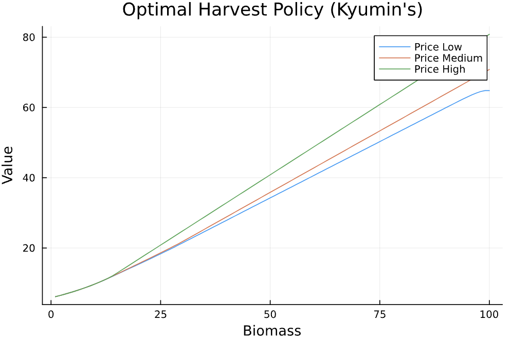
Figure 1: Value functions for each price state
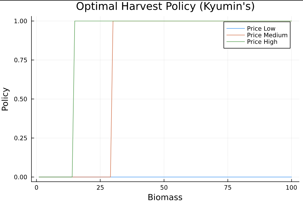
Figure 2: Optimal cut-versus-wait decision (1 = cut, 0 = wait)
8. Take-aways
- Encoding persistence with an MTM is clean for handling uncertainty—goodbye, Monte-Carlo integration.
- Price booms pull the trigger forward; slumps push it back.
- Uncertainty is not always a villain—it can turn resource modelling into an engaging puzzle box.
9. Julia Implementation
Here's the complete Julia code that implements the optimal tree harvesting model with Markov transition matrices:
#### Optimal Tree Harvest Control in Forestry ####
#### Author: Kyumin Kim ####
### Disclaimer: This is a simplified model for the purpose of showcasing optimal forestry control by MTM.
### Feel free to use this code for your own research, but I do not guarantee the accuracy of the results.

# Load essential packages
using Random, Interpolations, Optim, LinearAlgebra, Statistics  # general-purpose numerical packages                  # for graphing results
using Plots
using LinearAlgebra: dot


# model setup
b_max= 100; # maximum biomass of tree
c_cut= 5.0 # cost of cutting a tree

β= 0.95 # discount factor

#Now price has different possbility as random variable
price_val = [0.3, 0.7, 0.8]  # Low, Medium, High possibiltiy in the market.

#Transition probability matrix by AR(1) process. Column is the current state, row is the next state.
Π= [0.6 0.4 0.2;
0.3 0.4 0.3;
0.1 0.2 0.5]

Π[:,3]

#Okay let's define the state space: I one by one grid since biomass will increase by one
b_grid=1:1:b_max
num_biomass= length(b_grid)

#Price is also state variable
num_price= length(price_val)

# Bellman equation setup
max_iter= 2000
ϵ=1e-6


# initialize the value function and policy function to store
V_old=zeros(num_biomass, num_price) #Current value function
V_new=similar(V_old) #Next period value function
opt_policy=zeros(num_biomass, num_price) #Optimal policy function


#Now set bellman iteration

for iter in 1:max_iter

    for i in 1:num_biomass  #Over current biomass state
        for j in 1:num_price #Over current price state

            opt_value = -Inf
            opt_action =-Inf

            b= b_grid[i]
            p= price_val[j]


            ## action 1: cut
            immediate_reward = p * b - c_cut
            EV_cut = β * dot(Π[:,j],V_old[1, :]) # Since after cutting, biomass will be 1
            value_cut = immediate_reward + EV_cut


            ## action 0: wait
            next_biomass=min(b+1, b_max)
            value_wait = β * dot(Π[:,j],V_old[next_biomass, :])

            #Now compare the two values to find the optimal action

            if value_cut > value_wait
                opt_value = value_cut
                opt_action = 1
            else
                opt_value=value_wait
                opt_action = 0

            end

            V_new[i,j] = opt_value #Store the optimal value
            opt_policy[i,j] = opt_action  #Store the optimal action

        end
    end

    #Check convergence
    diff = maximum(abs.(V_new .- V_old))
    println("Iteration $iter, Difference: $diff")

    if diff < ϵ
        break
    end

    V_old .= V_new
end


# Plot the value function over biomass and each price state

plot(b_grid, V_new[:,1], label="Price Low", xlabel="Biomass", ylabel="Value", title="Optimal Harvest Policy (Kyumin's)")
#Add second plot in the second price state
plot!(b_grid, V_new[:,2], label="Price Medium")
plot!(b_grid, V_new[:,3], label="Price High")

# Add legend to explain which line corresponds to which price state
plot!(legend=:topright, bbox_to_anchor=(1.0, 1.0))

#Optimal policy over biomass and each price state
plot(b_grid, opt_policy[:,1], label="Price Low", xlabel="Biomass", ylabel="Policy", title="Optimal Harvest Policy (Kyumin's)")
plot!(b_grid, opt_policy[:,2], label="Price Medium")
plot!(b_grid, opt_policy[:,3], label="Price High")
plot!(legend=:topright, bbox_to_anchor=(1.0, 1.0))
This Julia implementation demonstrates the complete numerical solution to the optimal tree harvesting problem. The code includes the Bellman equation iteration, convergence checking, and plotting functions to visualize both the value functions and optimal policy rules.