Optimal Fisheries Management Under Uncertainty: Using Stochastic Dynamic Programming

1. Motivation

In the first part of this series, I solved an optimal fishing effort problem using dynamic programming under a fully deterministic setting. HOWEVER, the real world is not that clean—fish stocks fluctuate a lot! Fish populations grow unpredictably due to climate variability and ecological shocks, and these uncertainties are getting worse with accelerating climate change.

From a management perspective, this introduces serious risk. If we don't account for bad environmental shocks and act as if the fish stock is healthy, we might end up overfishing and pushing the stock toward collapse. So, yes, we need to explicitly deal with this climate risk.

To make our model more realistic, we now extend it to include stochastic growth—randomness in the fish stock dynamics. The goal is still the same: choose effort $E_t$ each year to balance current profits with the expected future value of the stock.

2. Model Ingredients

Stock Dynamics with a Multiplicative Shock

We introduce $\xi_t$, a random productivity shock, modeled as:

where in our simulation we set $\mu = -0.5$ and $\sigma = 0.3$. This means shocks are, on average, negative—climate-driven stress tends to reduce fish productivity—but occasionally we get a lucky year with a fish boom!

So the new (stochastic) stock dynamics become:

where $r$ is intrinsic growth rate, $K$ is carrying capacity, and $q$ is catchability—same as in the previous post, but now with randomness!

Profit Flow

Harvest is $h_t = q X_t E_t$. The immediate profit in a given year is:

where $p$ is the price per ton of fish and $c$ is the cost per unit effort.

Planner's Objective

Now the fishery planner maximizes the expected discounted sum of profits:

3. Bellman Equation

Let $V(X)$ be the value of being in state $X$. Then the Bellman equation is:

where $X'(\xi, E)$ is the next-period stock, and the expectation is taken over the stochastic shock $\xi$. Now, keep in mind that the future value function $V(X')$ is in the expectation operator!

4. Uncertainty and Monte Carlo Integration

• State discretization. We still use a grid for the fish stock state $X \in [X_{\min}, X_{\max}]$, dividing it into $n$ grid points.
• Continuous action space. Unlike before, we don't discretize fishing effort. Instead, we treat $E$ as continuous and use optimization algorithms (like Brent's method) to find the best effort.
• Monte Carlo integration. To evaluate the expectation over future value, we simulate $M$ shocks $\{\xi^{(m)}\}_{m=1}^M$ from the log-normal distribution:
  $$\mathbb{E} \big[ V(X'(\xi, E)) \big] = \int V(X')\, dF_{X'}(X') \approx \frac{1}{M} \sum_{m=1}^M V\big( X'(\xi^{(m)}, E) \big)$$
  This works thanks to the law of large numbers. As $M$ gets large, the average converges to the true expectation. Monte Carlo integral is simple to implement (a bit computationally heavy, but... easy-peasy, lemon squeezy 🍋). I'm a little lazy, so this works well for now! Of course, I'll show better integration tricks later on.
• Interpolation. Previously, we approximated value functions by snapping the next state to the nearest grid point. That sometimes gave jagged and spiky policies. Now we use interpolation to estimate $V(X')$ even when $X'$ is not on the grid. Here's how it works:

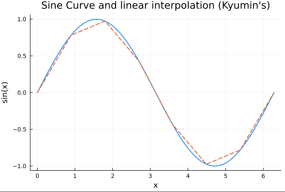
Figure 1: Linear interpolation example

You provide values at grid points, and interpolation fills in the rest. This makes the estimated value function smooth. I used linear interpolation here, but you can use fancier methods like cubic splines if needed. Which one's better? Depends! If your value function has sharp kinks, linear often works best.

Value function iteration.

1. For each stock level $X_i$, solve the maximization over effort $E$ (now a continuous variable).
2. Record the optimal effort $E^*(X_i)$ and the resulting value $V_{\text{new}}(X_i)$.
3. Update the value function and repeat until convergence.

5. Results

The value function looks pretty similar to the deterministic case. However, the numerical values are slightly lower—on average, our shock is bad (yikes!!). This reflects the negative impact of uncertainty.

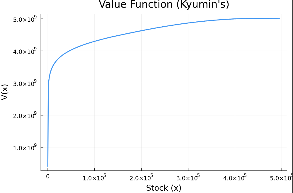
Figure 2: Value function under stochastic growth

Now that we use interpolation and continuous effort choice, our policy function (optimal fishing effort) is nice and smooth. No more spiky plot! Very satisfying.

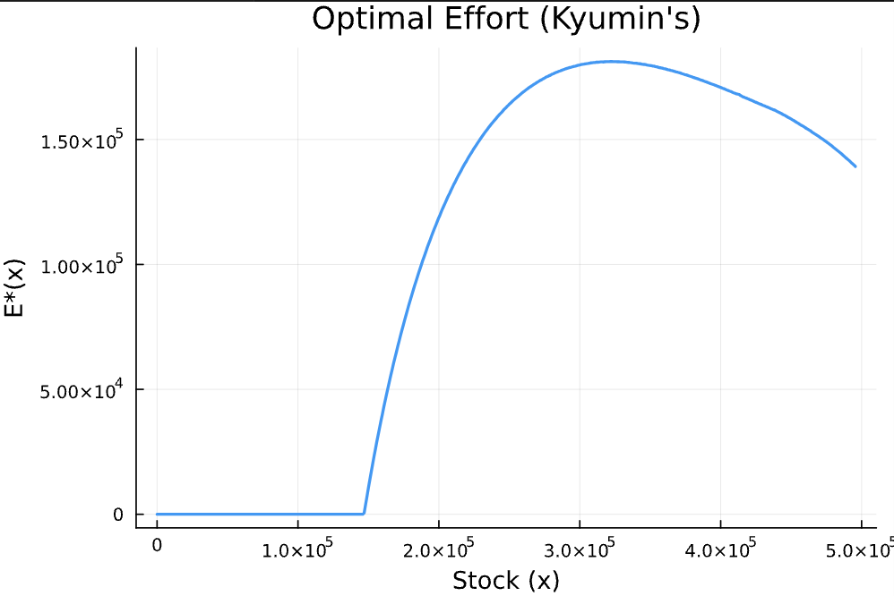
Figure 3: Optimal effort under stochastic dynamics

6. Stock Path Simulation Under Optimal Management

Well, this is stochastic dynamics for fish stocks. Even if we manage them under the found optimal fishing efforts policy, we should know what would happen in the future since each year, the shock and its impact is different every year. So let's do simulation. Over 100 years, under the optimal management, how the stock path would look? I repeated this simulation 100 times. The initial stock level is 20% of carrying capacity. And this is the results:

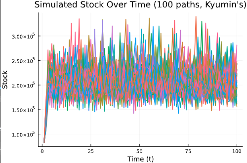
Figure 4: Stock path simulation under optimal management

Oh yeah, I found that after 100 years, and with 100 times of simulation, I didn't find bad cases where the stock is collapsed.

7. Conclusion

Adding stochastic growth and continuous effort control makes the model feel much closer to real life. Monte Carlo methods and interpolation make solving the model straightforward, even though uncertainty makes everything trickier. In future posts, I'll explore more sources of uncertainty—prices, costs, observation error, and maybe even multi-species models. After all, life (and fisheries!) is full of uncertainty.