The Value of Information from a Forecast: Inventory, Demand Uncertainty, and an Imperfect ML Signal
Business Decision Making Series 1
“The beauty of the universe, honestly, comes from chaos, not from order. If the cosmos returned the same outcome every time, like a machine, a hundred universes over, it would be unbearably boring.”
That is a line I am paraphrasing from a cartoon I watched as a kid, and it stuck with me for reasons I only understood much later: the interesting part of any system is the part we cannot perfectly predict.
I am a natural resource economist by training. But the thing that first pulled me into economics was never really fish or forests — it was uncertainty, and the question of how we are supposed to act well in the face of it. How do we read uncertainty, and how do we make a good decision under it, whether the uncertainty turns out to be good or bad? That question travels far beyond natural resources.
It almost became my dissertation. My first chapter was originally going to study how fishermen choose where to fish under uncertain information — uncertain stock distribution, and the risk of catching nuisance species like marine mammals that should never be caught. The information structure turned out to be far more tangled than I expected, and the data I needed did not exist, so the project became something else. But the underlying fascination never left me: how information shapes a decision, and what that information is actually worth.
As an applied economist I drift from my home research agenda fairly often, and I have come to think that is healthy. I care about natural resource economics, but I am just as drawn to production economics and to the mathematical programming side of operations research — in fact the methods in my own papers lean heavily on both. And lately, machine-learning forecasting and prediction are everywhere. When I read industry job descriptions, I keep noticing that “ML for forecasting” and “optimization” are treated as two separate specialties, owned by two separate kinds of people. That strikes me as exactly backwards. The people worth becoming, I think, are the ones who can fuse the two: ML to improve information, plus mathematical decision-making under uncertainty, plus dynamics, all in one head. That fusion is the thing I have been quietly trying to learn for a while now.
So today I picked a problem that lives right at that intersection. Inventory managementis a classic, almost mundane scheduling problem. But the moment you add dynamics and uncertainty — and especially once information starts to affect the decision structurally, through multiple layers of choice — it gets genuinely hard. And it is exactly the kind of place where a modern team would want to bolt an ML demand forecast onto the front of the decision. So that is the question for this post: a firm cannot see next period's demand, a machine-learning model whispers an imperfect guess about it, and we want to know — how much is that guess actually worth, in dollars? I will build a small infinite-horizon model where the answer can be computed exactly, and trace how the value of information rises with the accuracy of the forecast.
Julia code
Companion script: inventory_voi.jl. Requires Interpolations, Optim, Printf, and Plots. Run in Julia: include("inventory_voi.jl").
For more detailed guidance step by step, I attach a more detailed PDF version here.
Download PDF (inventory VOI guidance)Two Ways to Think About a Production Decision
Most introductory treatments of the firm are static: choose inputs (or output) once, set marginal revenue equal to marginal cost, and you are done. That picture is clean, but it quietly assumes two things that rarely hold in practice. First, that the firm knows the demand it faces. Second, that what it produces this period has no bearing on next period.
Relax both assumptions and the problem becomes genuinely dynamic. Demand arrives as a random shock; the firm can build a buffer of inventory to smooth the bumps; and the inventory it carries forward is a state variable that links today to tomorrow. This is the world of the classic production-smoothing literature, and it is also the natural place to ask a very modern question: if I bought a better demand forecast, how much would my profits rise?
I find this question appealing because it sits exactly on the seam between economic theory and machine learning. An ML team will happily report that their classifier is “85% accurate.” A decision maker wants to know what that buys. The bridge between the two is an old idea from decision theory — the value of information — embedded inside a dynamic optimization problem.
The Setup
A monopolist lives forever and discounts the future at rate . Time is discrete. Within each period the timing is what makes this an information problem, so it is worth stating carefully:
- The firm begins the period holding inventory (this is the state).
- It observes a machine-learning signal about demand — but the true state is not yet known.
- It chooses production at constant unit cost .
- The true demand multiplier is realised.
- It chooses sales , constrained by what it physically has: .
- Leftover stock carries forward, , and incurs a convex holding cost.
The reason production is decided before the state is realised, while sales are decided after, is the whole point. Information has value only because the firm must commit to under uncertainty. A better signal lets it commit better.
Demand is a high or low multiplicative shock, drawn i.i.d. across periods:
so a good year lifts the demand intercept by 30% and a bad year cuts it by 20%. The three primitive functions are deliberately simple:
The inverse demand is linear (so marginal revenue is linear and the algebra stays readable). The production cost is linear — this is exactly the constant-marginal-cost case you get from a constant-returns-to-scale Cobb-Douglas technology, where the unit cost is pinned down by factor prices. The holding cost is convex, and that convexity is what keeps the inventory problem alive.
Why convex holding cost, and not convex production cost? Both can motivate holding inventory. The textbook production-smoothing model puts the curvature in , so the firm spreads production over time. Here I keep the CRS production cost linear (constant marginal cost) and put the curvature in the holding cost instead. The economic story then becomes: it is fine to produce a lot in one burst, but piling stock into the warehouse gets expensive fast. That maps the value of information cleanly onto a single question — when should I build a buffer? — rather than smearing it across the production schedule.
Where the Information Lives: From Confusion Matrix to Posterior
An ML team would summarise a binary classifier with a 2×2 confusion matrix. Two numbers from it carry all the decision-relevant content:
But the firm does not act on the confusion matrix directly. When it sees a signal, it needs the probability that the underlying state is good given that signal. That is a posterior, and Bayes' rule delivers it:
The two extremes are the sanity checks that anchor everything below. A perfectclassifier () makes the posterior degenerate — the signal is the truth. A useless classifier (a coin flip, ) makes the posterior collapse back to the prior — the signal tells you nothing you didn't already know. Every classifier in between lands the posterior somewhere on the segment between “prior” and “truth,” and that position is precisely the lever that sets the value of information.
The Bellman Equation
Because the demand shock is i.i.d., next period's signal is independent of everything decided this period. That has a convenient consequence: the belief never becomes part of persistent state. The only thing the firm carries across periods is physical inventory . The signal matters within the period and then is gone. (This is the payoff of the i.i.d. assumption; with persistent demand the belief would enter the state and we would be in genuinely harder territory.)
Write the continuation value as . Before splitting the problem into stages, it is useful to write one nested Bellman equation that respects the timing: the firm sees the signal, commits to production , then learns and chooses sales :
The outer is the production decision (taken under the signal, before is known); the inner is the sales decision (taken after is realised, with available stock ). Current-stock holding cost depends on alone, so it sits outside both maximisations.
Because the inner problem depends on only through available stock , we can fold the sales stage into a subproblem and rewrite the Bellman as a two-stage problem. After the true state is realised and the firm holds available stock , the sales subproblem is
Substituting for the inner sales stage, the production problem becomes
Swapping out what the expectation conditions on is the only thing that changes across the three information regimes:
| Regime | Belief used to choose |
|---|---|
| No information | the prior |
| ML signal | the posterior implied by |
| Perfect information | the true (so is chosen knowing the state) |
Solving It: Continuous-State Value Function Iteration
Since , the Bellman operator is a contraction, so value function iteration converges to the unique fixed point from any starting guess. The implementation follows the standard recipe for a continuous state. I store the value function on a grid over inventory , and recover at off-grid points by linear interpolation (Julia's Interpolations.jl, with flat extrapolation at the boundaries). Production and sales are genuinely continuous choices, each solved by a bounded scalar optimiser (Optim.jl, Brent's method). This keeps the choices off the grid — the grid only discretises the state.
The sales subproblem is solved directly whenever the production search needs it, evaluated at available stock . There is no separate grid over and no cached table: is just an intermediate quantity, never a state variable. The single state is inventory , so the value function is genuinely one-dimensional. The outer loop is short:
function solve_vfi(P, regime; alpha=1.0, beta=1.0)
    Sg = state_grid(P)
    V  = zeros(P.nS)
    for it in 1:P.maxiter
        Vnew = bellman(P, Sg, V, regime, alpha, beta)
        diff = maximum(abs.(Vnew .- V))   # sup-norm
        V = Vnew
        diff < P.tol && break             # contraction guarantees this fires
    end
    return Sg, V
end
Inside bellman, for each state we choose by maximising with a one-dimensional Optim call, and each evaluation of is itself a one-dimensional Optim call over — the sales problem solved on the spot. The current-stock holding cost is additive and sits outside both optimisations. The full annotated source is in the companion script. (Caching on a grid of values would trade a little accuracy for speed; I keep the call direct because it is simpler and exact.)
A note on the kink. The sales constraint can bind in the good state, which puts a kink in the policy. Linear interpolation handles the value function well here because stays concave and smooth; the kink lives in the policy, not in . I verified the solution against an independent grid-consistent implementation (where and move in grid units so no interpolation is needed): the two agree to within grid resolution, which is the reassurance you want before trusting the numbers below.
Result 1: A Good Forecast Moves Production at Every Inventory Level
Before pricing the forecast, it helps to watch it act. The cleanest way to see this is the production policy — how much the firm makes as a function of the inventory it starts the period with — traced out separately for each information regime. Under the signal regime I plot the ex-ante policy: the production the firm commits to after seeing the signal but before demand is realized, averaged over which signal fires.
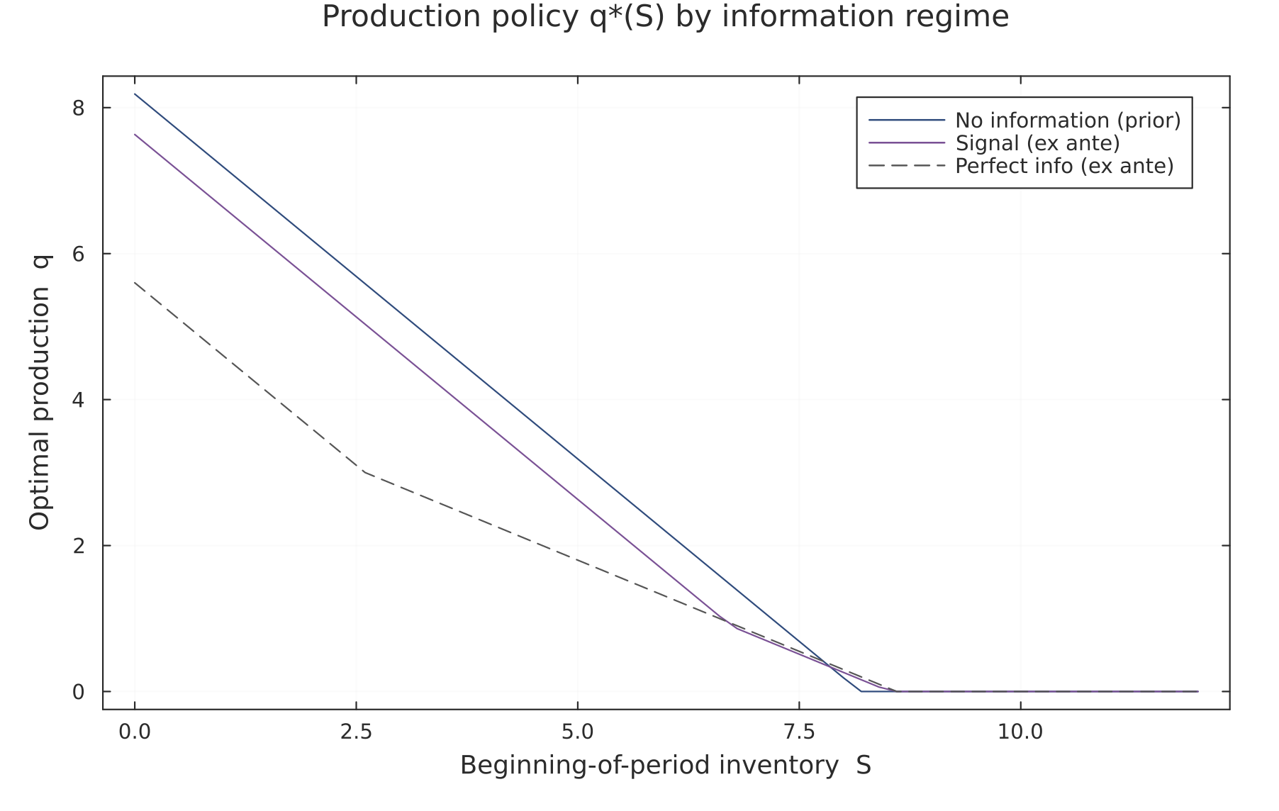
Figure 1. Optimal production across information regimes, as a function of beginning-of-period inventory . The firm produces less as it starts with more stock (it already has a buffer). Note the ordering of the three curves: no-information production is highest, the signal regime lower, and perfect information lowest. The empty-warehouse case () is just the left endpoint of each curve.
The striking feature is not just that the curves are ordered, but which way: the firm produces less, not more, as information improves. The reason is precautionary overproduction. Without a forecast, the firm hedges against the chance of strong demand by building a buffer it might not sell; when demand then turns out weak, that buffer becomes unsold stock carrying a holding cost. A forecast lets the firm trim that hedge, and perfect information removes the need for it almost entirely, since the firm makes only what it knows it can sell. So here the value of information shows up less as “selling more” and more as “wasting less”: it shrinks the defensive over-build rather than expanding output. That this is the dominant channel is a property of the payoff structure, the same asymmetry that, as we will see, makes the efficiency map lean toward the true positive rate.
Result 2: Where the Value Lives — Value Functions and State-wise VOI
The value of information is, by definition, the vertical gap between value functions. Plotting for all three regimes makes that gap visible at every inventory level, and the difference is the value of information, state by state.
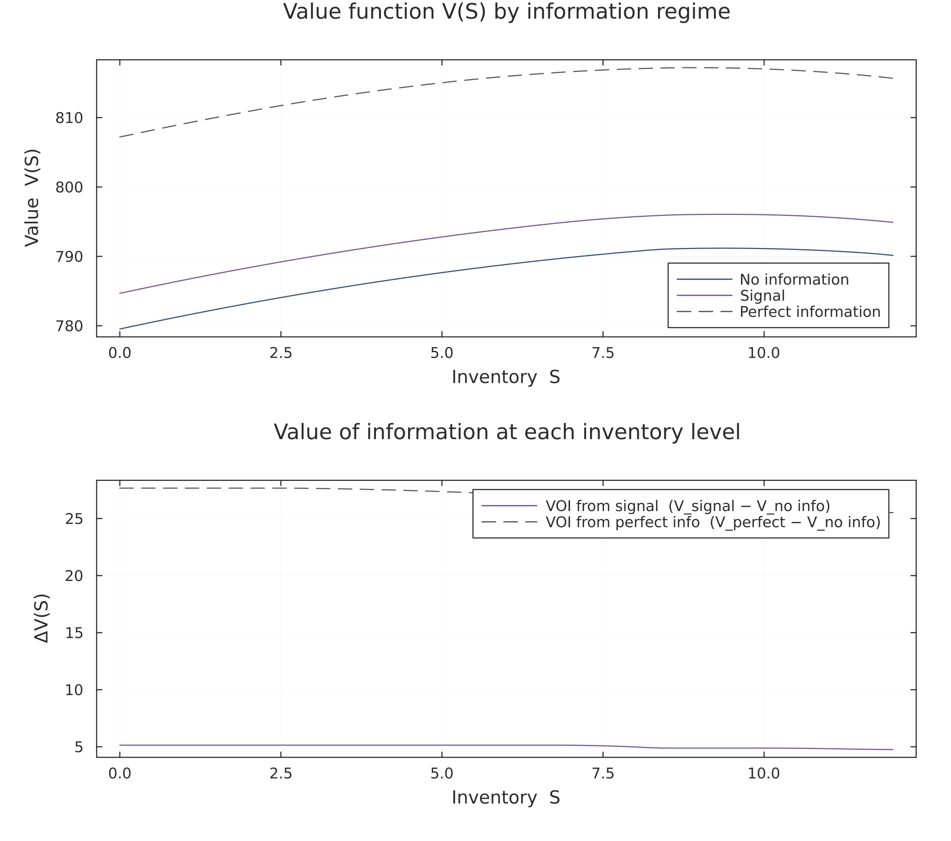
Figure 2. Top: the value function under each regime; the curves sit in the order everywhere, since more information is always weakly better. Bottom: the value of information at each inventory level — the signal's worth (solid) and the perfect-information ceiling (dashed). Reading these two panels together shows not just how much information is worth, but where (at which inventory levels) it matters most.
For a headline number, evaluate these at the empty-warehouse reference point (classifier TPR = TNR = 0.85, high-VOI parameters from the companion script):
| Quantity (present value, at ) | Value |
|---|---|
| — no information | 779.5376 |
| — ML signal (TPR = TNR = 0.85) | 784.6767 |
| — perfect information | 807.2000 |
| VOI of the signal | 5.1392 |
| VOI of perfect information | 27.6624 |
| Efficiency (share of perfect-info value captured) | 18.6% |
These numbers come from running inventory_voi.jl with the high-VOI parameter set (high_voi_params()). The figures and these numbers are generated from the same run so they agree. Each is a present value — the discounted sum of all future profits, not a single period's profit — so the VOI figures are present values too.
Result 3: Pricing the Forecast — VOI Rises with Accuracy
Sweeping the classifier's accuracy from a coin flip to perfection traces out the value of the forecast. At accuracy 0.5 the signal is worthless and VOI is exactly zero — the posterior collapses to the prior, so the firm behaves as if it had no signal at all. At the other end, a perfect forecast hits the ceiling by construction.
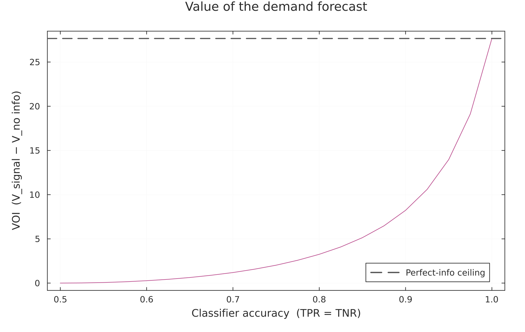
Figure 3. The value of information as a function of symmetric classifier accuracy (TPR = TNR), with the perfect-information ceiling marked as a dashed line. VOI starts at zero for a useless classifier and climbs toward the ceiling as the forecast sharpens; the curvature tells you how the returns to forecast quality are distributed across the accuracy range.
The managerial reading is blunt: a barely-better-than-random classifier captures almost none of the available value, because its posterior hardly moves from the prior, so the firm hardly changes its behavior, so it hardly captures any gains. How much of the value is back-loaded toward high accuracy is exactly what the shape of this curve reveals for your parameters.
Result 4: Not All Accuracy Is Equal
So far I forced the classifier to be symmetric (TPR = TNR). Letting the two rates vary separately reveals an asymmetry that a single “accuracy” number would hide.
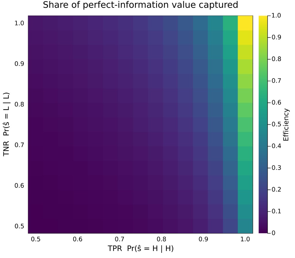
Figure 4. Share of perfect-information value captured, over the true positive rate (horizontal) and true negative rate (vertical). If the contours lean closer to vertical than to horizontal, efficiency responds more strongly to TPR — correctly flagging the gooddemand state — than to TNR; a horizontal lean means the reverse.
Which way the heatmap tilts is decided by the payoff structure, not by the classifier. When the cost of being caught short in a good state (under-producing, leaving profitable sales unmet) outweighs the cost of over-producing into a bad state (a bounded, convex holding cost), the firm values a signal that reliably calls the upside, and the heatmap leans toward rewarding TPR. The practical implication is that, if you can only improve one dimension of your model, the economics — not the confusion matrix — should tell you which one.
What I Take Away From This
The exercise is small, but it makes three things concrete that are easy to wave at and hard to pin down. It gives the value of an imperfect forecast an actual number, in the same profit units the firm already cares about. It shows that the relationship between statistical accuracy and economic value is convex, not linear — so “how accurate is the model?” is the wrong question without “and how does accuracy map to decisions?” And it shows that the two error types are not interchangeable: the structure of the payoff decides which kind of mistake is more expensive.
None of this requires exotic machinery — just a contraction mapping, Bayes' rule, and a willingness to be explicit about timing. That, to me, is the appeal of writing the model down: it turns a vague intuition (“better forecasts help”) into a quantity you can compute, plot, and argue about.
And it closes the loop on where I started. The forecast is the source of uncertainty here, but a good forecast does not remove the uncertainty — it just reshapes it into something the firm can act on more wisely. The interesting decisions still live in the part we cannot perfectly predict. What this little model does is let the two halves I care about — the ML forecast that improves information, and the dynamic optimization that acts on it — sit inside a single objective, where each can be priced against the other. That fusion, far more than the specific numbers, is what I wanted to show.
Reproduce everything
The companion script solves all three regimes by value function iteration and regenerates the accuracy curve and the efficiency heatmap.
Download inventory_voi.jl