Machine Learning Series 4: Random Forest Hyperparameters and Practical Grid Search

Why Hyperparameters Matter

When people say Random Forests are "robust," they usually mean two things: they work reasonably well with minimal tuning, and they do not fall apart if your settings are not perfect. That rule of thumb is mostly true—but not the whole story. Accuracy and stability still hinge on a few key choices. With a small, sensible grid, you can often squeeze out a clear improvement without heavy compute.

Parameters vs. Hyperparameters (at a Glance)

Parameters are learned from the data during training (e.g., split points and leaf values inside each tree). Hyperparameters are settings you choose before training that shape how the model learns (e.g., number of trees, features per split, and leaf limits). In this post we focus on tuning those hyperparameters.

Parameters vs. Hyperparameters

In machine learning, parameters are numbers the model learns from the data. In linear regression, the slope and intercept are parameters. In a Random Forest, there are no global slopes to learn, but each tree learns split points and region means. Those are learned automatically during training.

Hyperparameters are the settings you choose before training that shape how the learning happens. They are not learned from the data unless you run a tuning procedure. In Random Forests, the useful ones are:

• n_estimators (ntree): how many trees to grow.
• max_features (mtry): how many predictors each split is allowed to look at.
• max_leaf_nodes (maxnodes): the maximum number of terminal nodes per tree.
• nodesize: the minimum number of observations required in a leaf.

Choosing these is like setting the rules of the game before the trees start growing. Again, the choice of those hyperparameter values are all about bias-variance tradeoff for predictions.

The Bias–Variance Tradeoff in Plain Language

Every predictive model balances two kinds of error:

• Bias: error from a model that is too simple. Think of a ruler trying to trace a curvy line.
• Variance: error from a model that is too sensitive to the sample. Think of tracing every tiny wiggle in the line, including noise.

Random Forests reduce variance by averaging many trees. Two choices help a lot:

• More trees (n_estimators) lower variance. In general, returns diminish after a point and training time increases, so we look for a plateau—so once it reaches flat regions for improvement, well, benefits from more tree would be marginal.
• Feature subsampling (max_features) decorrelates trees. Smaller values make trees look at different slices of the data, which usually helps generalization. Too small can raise bias.

To keep bias under control, we also cap tree complexity:

• Leaf limits (max_leaf_nodes) and minimum leaf size (nodesize) act as regularizers to balance between overfitting and underfitting.

Hyperparameters Tuned

We focus on four levers that most influence predictive performance in practice:

• n_estimators (ntree): number of trees. More trees reduce variance with diminishing returns. Training time grows roughly linearly.
• max_features (mtry): number of predictors considered at each split. Smaller values decorrelate trees and often improve generalization. Too small can increase bias.
• max_leaf_nodes (maxnodes): upper bound on terminal nodes per tree. Controls global tree complexity and helps prevent overfitting.
• nodesize: minimum observations per leaf. In this post we fix it at 5 so that effects of the three knobs above are clear.

Evaluation Protocol

We use a single 50/50 train and test split to keep comparisons fixed.

• OOB MSE and OOB $R^2$ are internal yardsticks during the sweep.
• Test RMSE (log scale) on the holdout set is the final selection criterion.

Results

Below are the results from a grid search over 100 combinations of hyperparameters. Figure 1 reports the top ten Random Forest settings ranked by holdout Test RMSE (log scale). We could also rank models by the out-of-bag (OOB) MSE—a bootstrap-based, cross-validation–like estimate computed during training—but to keep the focus clear, we evaluate final models by Test RMSE on the holdout set.

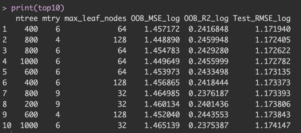
Figure 1: Top ten hyperparameter settings ranked by holdout Test RMSE (log scale). When multiple settings are statistically indistinguishable, prefer the simpler model.

When several models achieve similar Test RMSE, a practical rule of thumb is to choose the simpler one: fewer trees, smaller leaf budgets, or a smaller mtry. This usually saves computation and memory without sacrificing accuracy.

If many hyperparameters must be tuned simultaneously (especially with fine-grained grids), an exhaustive grid over all combinations can become computationally expensive. In such cases, random search is an efficient alternative: instead of evaluating every point on a global grid, you sample hyperparameter values at random from reasonable ranges. Random search explores more distinct settings in the same compute budget and often finds strong configurations quickly. (It has trade-offs, of course; we will cover them in a future post.)

Conclusion

Hyperparameter tuning is a crucial step in maximizing Random Forest performance. While Random Forests are often considered robust out-of-the-box, systematic tuning can lead to meaningful improvements in prediction accuracy. The key is to balance exploration with practical constraints—a compact grid search often suffices to find strong settings.

The results from our grid search demonstrate that different hyperparameter combinations can yield similar performance, validating the importance of choosing simpler models when performance is comparable. This approach not only saves computational resources but also improves model interpretability and deployment ease.

R Code Implementation

Below is the complete R code used to perform the grid search and generate the results presented in this post.

##### RF tuning with log target (ltotexp) #####

# install.packages(c("haven","dplyr","randomForest")) # if needed
rm(list = ls())

library(haven)
library(dplyr)
library(randomForest)

# ---- Load & filter ----
dat <- read_dta("/Users/kyuminkim/Google Drive/ML example/mus203mepsmedexp.dta") %>%
  filter(!is.na(ltotexp))

# Predictors
xlist <- c("income","educyr","age","famsze","totchr")
dlist <- c("suppins","female","white","hisp","marry","northe","mwest","south",
           "msa","phylim","actlim","injury","priolist","hvgg")
preds <- c(xlist, dlist)

# Modeling DF
df <- dat %>%
  select(totexp, ltotexp, all_of(preds)) %>%
  mutate(across(all_of(dlist), ~ as.factor(.)))

# Train / Test split (50/50)
set.seed(10101)
train_idx <- sample.int(nrow(df), size = floor(0.5 * nrow(df)))
train <- df[train_idx, ]
test  <- df[-train_idx, ]

# Helpers
p <- length(preds)
rmse <- function(y, yhat) sqrt(mean((y - yhat)^2))

# -------------------------------
# Grid definition
# -------------------------------
ntree_grid <- c(200, 400, 600, 800, 1000)

mtry_candidates <- c(floor(p/3), floor(sqrt(p)), floor(p/2), p)
mtry_candidates[mtry_candidates < 1] <- 1
mtry_candidates[mtry_candidates > p] <- p
mtry_grid <- sort(unique(mtry_candidates))

max_leaf_nodes_grid <- c(NA, 32, 64, 128, 256)

grid <- expand.grid(
  ntree = ntree_grid,
  mtry = mtry_grid,
  max_leaf_nodes = max_leaf_nodes_grid,
  KEEP.OUT.ATTRS = FALSE,
  stringsAsFactors = FALSE
)

# -------------------------------
# Fit & evaluate for each combo
# -------------------------------
set.seed(20251010)

run_one <- function(ntree, mtry, max_leaf_nodes) {
  maxnodes_arg <- if (is.na(max_leaf_nodes)) NULL else as.integer(max_leaf_nodes)

  fit <- randomForest(
    ltotexp ~ ., data = train[, c("ltotexp", preds)],
    ntree = ntree,
    mtry = mtry,
    nodesize = 5,
    maxnodes = maxnodes_arg,
    importance = TRUE,
    keep.forest = TRUE
  )

  oob_mse <- if (!is.null(fit$mse)) tail(fit$mse, 1) else NA_real_
  oob_rsq <- if (!is.null(fit$rsq)) tail(fit$rsq, 1) else NA_real_

  pred_test_log <- predict(fit, newdata = test[, preds, drop = FALSE])
  test_rmse_log <- rmse(test$ltotexp, pred_test_log)

  list(fit = fit, oob_mse = oob_mse, oob_rsq = oob_rsq, test_rmse_log = test_rmse_log)
}

cat(sprintf("Total combos: %d\n", nrow(grid)))

results_list <- vector("list", nrow(grid))
for (i in seq_len(nrow(grid))) {
  g <- grid[i, ]
  out <- run_one(ntree = g$ntree, mtry = g$mtry, max_leaf_nodes = g$max_leaf_nodes)
  results_list[[i]] <- cbind(g, data.frame(
    OOB_MSE_log   = out$oob_mse,
    OOB_R2_log    = out$oob_rsq,
    Test_RMSE_log = out$test_rmse_log,
    stringsAsFactors = FALSE
  ))
  if (i %% 10 == 0) cat(sprintf("... %d/%d done\n", i, nrow(grid)))
}

results_df <- dplyr::bind_rows(results_list)

# Top 10 by Test RMSE (log)
top10 <- results_df %>%
  arrange(Test_RMSE_log) %>%
  mutate(max_leaf_nodes = ifelse(is.na(max_leaf_nodes), "None", as.character(max_leaf_nodes))) %>%
  select(ntree, mtry, max_leaf_nodes, OOB_MSE_log, OOB_R2_log, Test_RMSE_log) %>%
  head(10)

print(top10)

# Best model refit
best_row <- results_df %>% arrange(Test_RMSE_log) %>% slice(1)
best_maxnodes <- if (is.na(best_row$max_leaf_nodes)) NULL else as.integer(best_row$max_leaf_nodes)

set.seed(20251010)
best_model <- randomForest(
  ltotexp ~ ., data = train[, c("ltotexp", preds)],
  ntree = best_row$ntree,
  mtry = best_row$mtry,
  nodesize = 5,
  maxnodes = best_maxnodes,
  importance = TRUE,
  keep.forest = TRUE
)

cat("\nBest combo (log target):\n")
print(best_row %>% select(ntree, mtry, max_leaf_nodes, OOB_MSE_log, OOB_R2_log, Test_RMSE_log))

# Importance plot (export for Figure 3)
imp_best <- importance(best_model)
v_best <- sort(imp_best[, "IncNodePurity"], decreasing = TRUE)
scale_importance <- function(x) 100 * x / max(x, na.rm = TRUE)
v_scaled <- scale_importance(v_best)

barplot(v_scaled, las = 2, cex.names = 1.0,
        main = sprintf("Variable Importance (Best RF, log target)\nntree=%d, mtry=%d, maxnodes=%s",
                       best_row$ntree, best_row$mtry,
                       ifelse(is.na(best_row$max_leaf_nodes), "None",
                              as.character(best_row$max_leaf_nodes))),
        ylab = "Relative Importance (0–100)")

# Optional: export figures
# png("importance_best.png", width=900, height=600); <barplot code>; dev.off()
# png("grid_overview.png",  width=900, height=600); # your grid heatmap; dev.off()
# png("top10_results.png",  width=900, height=600); # your top10 chart; dev.off()