Kyumin Kim | Fisheries and Emission Cost: Addressing Economic Uncertainty through Monte Carlo Simulation: Series 2

Disclaimer: This analysis, from an economics perspective, has several limitations regarding its practical implications. Today's focus is primarily on the technical application of Monte Carlo simulation to handle economic uncertainty.

In my previous post "Optimal Fishing Management Under Emission Cost in Korean Fisheries: Series 1," we found that economically efficient fishing involves applying less fishing effort compared to the "race-to-fish" approach of excessive fishing. This creates a triple win: higher fishing profits, lower GHG emissions, and healthier fish stocks!

In that previous deterministic analysis, we calculated optimal fishing effort as a function of several parameters: fish price ( $p$ ), biological conditions of fish stocks ( $a,b$ ), fishing cost ( $c$ ), and emission costs ( $e$ ) involved in purchasing emission credits in the Emission Trading Scheme (ETS) market. Under the hypothetical setup where fisheries are now managed under an Emission Trading Scheme (ETS), as a reminder from the previous posting in series 1, the optimal fishing effort is given by:

E_{\text{MEY}}^{\text{ETS}} = \frac{pa - (c + e)}{2pb}

In economics, expressing solutions as functions of parameters is natural. When you solve for an optimal solution and a closed-form analytical solution is available, it's expressed as a function of the model's given parameters. This relates to the Envelope Theorem in economic theory.

However, this equation shows that optimal fishing effort varies significantly depending on economic conditions characterized by these parameters. In reality, all parameters fluctuate over time, and we often don't know which economic scenario will actually occur. This is where uncertainty becomes crucial! For instance, assuming that emission costs or fish prices remain fixed is unrealistic. Therefore, point estimates of optimal fishing efforts may be less reliable.

To address this limitation, we can adopt a probabilistic perspective by quantifying uncertainty and exploring different possible outcomes. I conducted a Monte Carlo simulation treating each parameter as a random variable with its own probability distribution.

Instead of treating economic variables like fish price and emission costs as fixed values, we now consider them as random variables with multiple possible realizations. How do we characterize this uncertainty? Through probability distributions!

Once we know each random variable's distribution, we can simulate how our optimal solution behaves under economic uncertainty. Figure 1 illustrates the Monte Carlo simulation concept: iteratively draw values from probability distributions, run simulations, and observe the distribution of results.

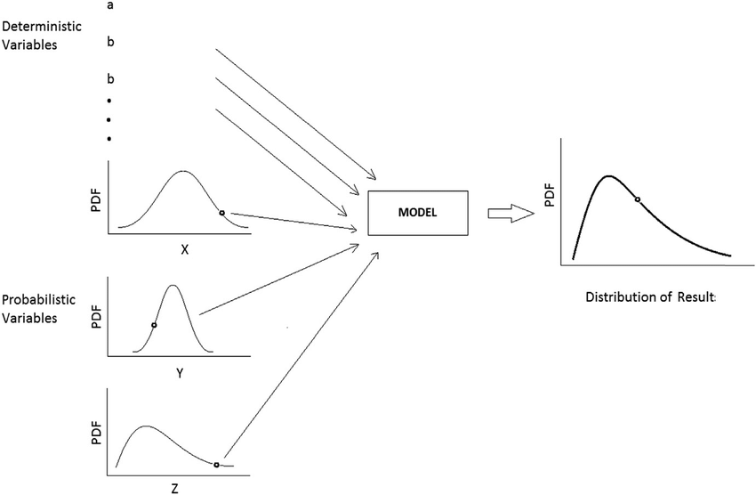
Figure 1: Schematic of Monte Carlo simulation. (Source: Vu et al. 2018, Probabilistic analysis and resistance factor calibration for deep foundation design using Monte Carlo simulation)

1. Parameter Distributions: Choosing Appropriate Distributions for Uncertainty

You might wonder: what distribution should I use to characterize uncertainty? There are multiple approaches. One method I used involves fitting empirical distributions (real-world data) to theoretical distributions.

For example, I fitted my empirical distribution of anchovy fish price data (approximately 180 monthly domestic anchovy price observations in Korea) to a theoretical distribution. After testing 32 different probability distributions on the price dataset, I found that the gamma distribution provided the best fit to the empirical data. The gamma distribution is characterized by two parameters: shape and scale. In our case, the price data fitted to Gamma(α=4.62 (shape), β= 0.002 (scale)).

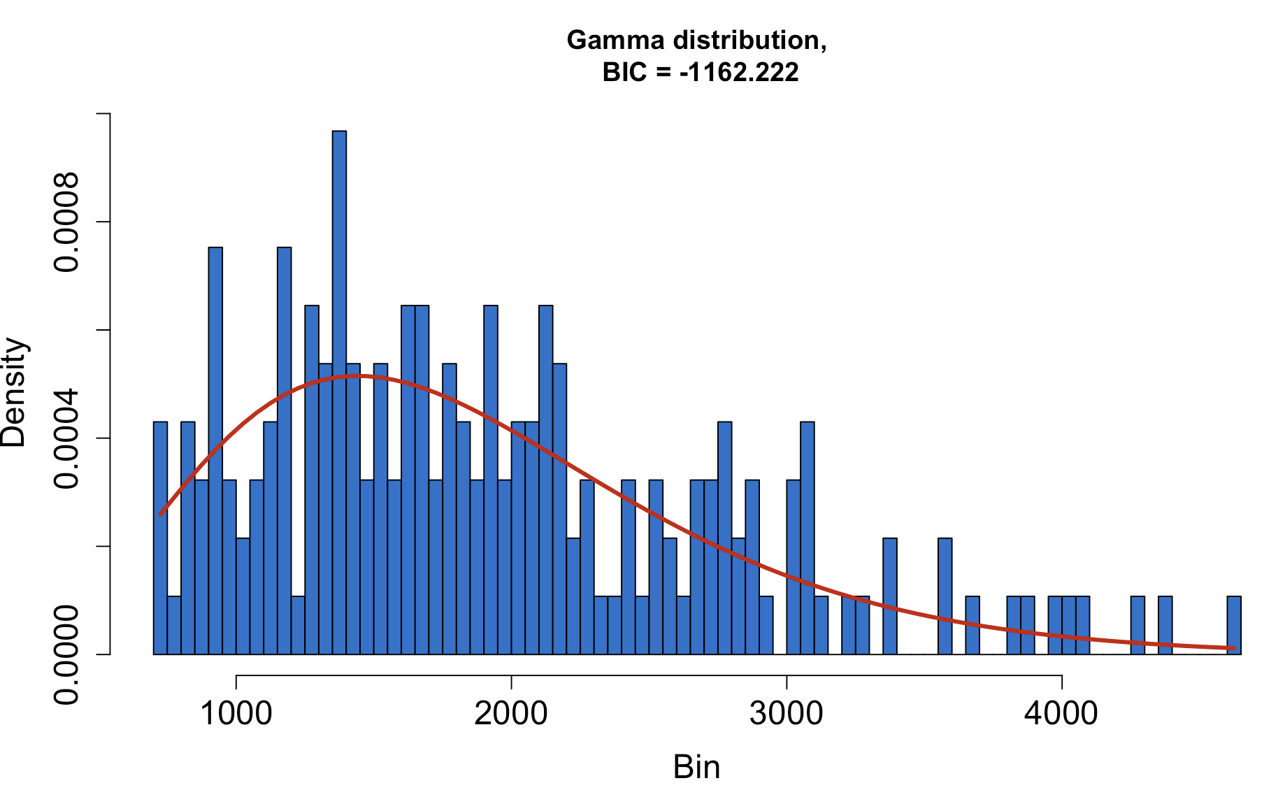
Fish price data fitted to Gamma Distribution

Figure 2: Fish price data ( $p$ ) fitted to Gamma Distribution ( $\text{Gamma}(\hat{\alpha},\hat{\beta})$ )

Technical note: I found the optimal shape and scale parameters by minimizing the Kullback-Leibler divergence, which quantifies the difference between the assumed distribution and the empirical data:

\hat{\alpha}, \hat{\beta} = \arg\min_{\alpha,\beta} \sum_{i=1}^{n} \hat{p}(x_i) \log \frac{\hat{p}(x_i)}{q_{\alpha,\beta}(x_i)}

where $q$ represents the specified gamma distribution $\text{Gamma}(\alpha,\beta)$ , $\hat{p}$ represents the empirical data, $i$ indexes individual data points, and $n$ is the total number of observations.

I applied the same process to other economic parameters:

p \sim \text{Gamma}(4.623, 0.00251)

(fish price per ton)

\text{GHG} \sim \text{Triangular}(0.624, 0.844, 0.813)

(emissions (

\text{CO}_2\text{eq}

) per HP)

c_{emi} \sim \text{Cauchy}(21.07, 3.71)

(carbon credit price per ton

\text{CO}_2\text{eq}

)

c \sim \text{Triangular}(187, 508, 301)

(fishing cost per HP)

a = 1.38

(fixed biological parameter)

b = 3.84 \times 10^{-6}

(fixed biological parameter)

The emission cost per unit effort is: $e = \text{GHG} \times c_{emi}$ . For GHG and fishing cost ( $c$ ), I used triangular distributions due to limited data availability. Triangular distributions are commonly used when data observations are limited but you know the minimum value (lower bound), maximum value (upper bound), and mode (most likely value).

2. Simulation Process

For each Monte Carlo iteration $i = 1, ..., 5000$ with $N = 400$ samples per iteration (these numbers were chosen somewhat arbitrarily for computational convenience), the process works as follows:

Draw random values from each parameter distribution
Calculate $E_{\text{MEY},i}^{\text{ETS}} = \frac{p_i \cdot a - (c_i + \text{GHG}_i \cdot c_{emi,i})}{2 \cdot b \cdot p_i}$ and other relevant measures (emission costs, emission savings, profits) at the sampled optimal fishing effort
Store the results

This process generates probability distributions of optimal fishing efforts, GHG emissions, and profits under economic uncertainty, rather than single point estimates.

3. Results

Now we can examine the distributions of key outcomes under economic uncertainty (i.e., varying economic conditions including fishing prices, emission credit prices in the ETS market, unit emission rate, and fishing cost).

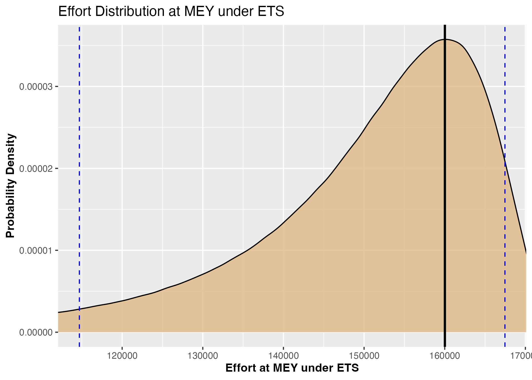
Figure 3a: Probability density distribution of optimal fishing efforts under ETS scenario

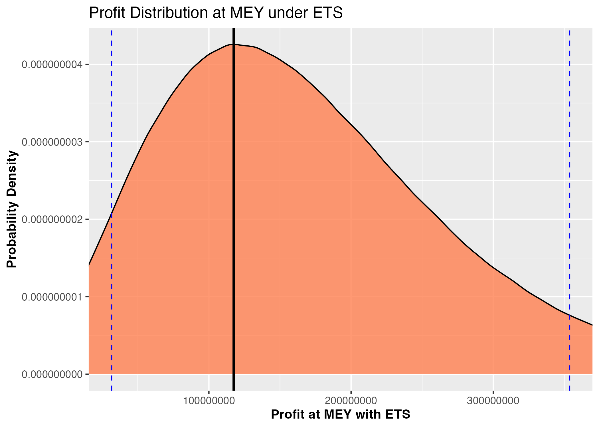
Figure 3b: Probability density distribution of fishing profits under optimal fishing efforts and ETS scenario

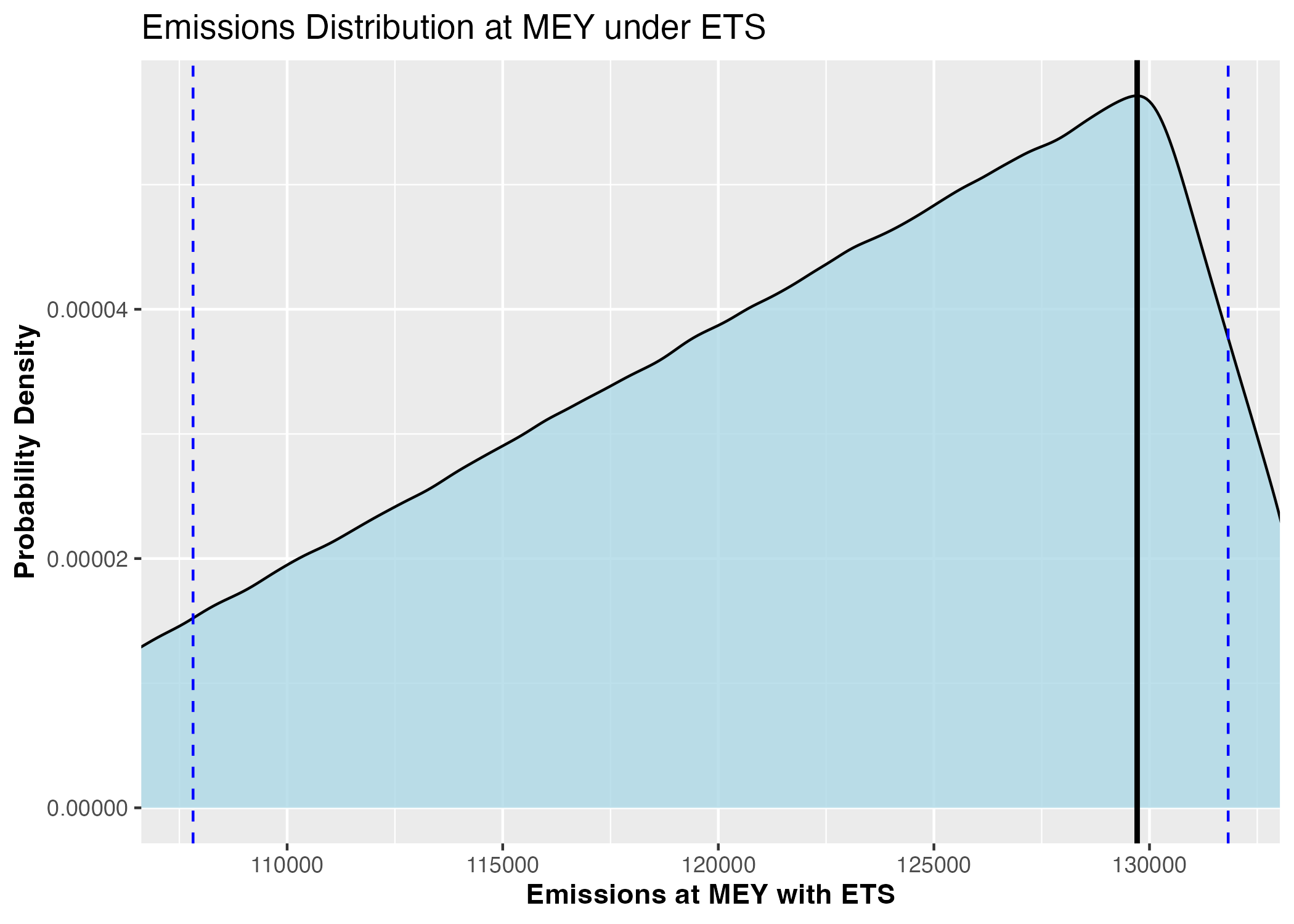
Figure 3c: Probability density distribution of GHG emissions under optimal fishing efforts and ETS scenario

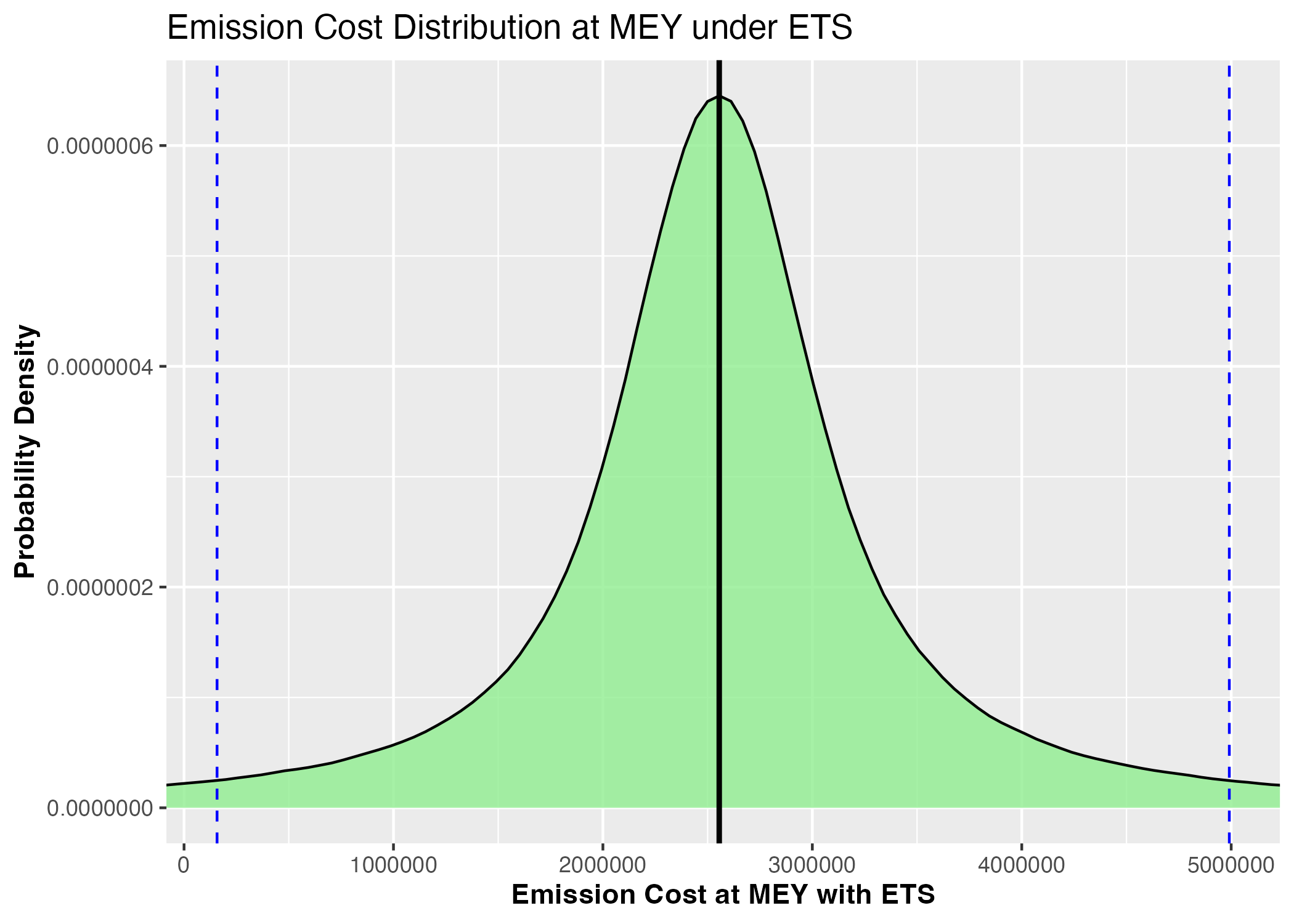
Figure 3d: Probability density distribution of emission costs under optimal fishing efforts and ETS scenario

Figure 3: Monte Carlo simulation results under Emission Trading Scheme incorporated in optimal economic fishing management: optimal fishing efforts, profit outcomes, emission levels, and associated costs (Blue dashed lines represent 90% confidence intervals)

4. Statistical Inference

This approach provides policymakers with complete probability distributions of outcomes rather than just point estimates, enabling risk-informed decision making. For instance, we can now state "with 90% confidence, optimal fishing efforts will result in profits, emissions, and emission costs within specific ranges under considering economic uncertainty of price of fish, cost of fishing and emission" rather than providing single deterministic values.

The Monte Carlo analysis confirms that even under economic uncertainty (characterized by parameter uncertainty), reducing fishing effort to Maximum Economic Yield (MEY) levels remains both economically and environmentally beneficial, with probabilistically quantifiable outcome ranges.

Code Implementation: I've provided the complete R code that implements this Monte Carlo simulation. The code generates all the figures shown above and performs the full uncertainty analysis.

R Implementation

# Monte Carlo Simulation for E_MEY under an ETS Scenario

#########################################################################################
# Disclaimer: This code is a prototype and provided as-is, with no guarantees of       #
# correctness or technical accuracy. You are free to use and modify this script for    #
# your own purposes. However, please be aware that the author takes no responsibility  #
# or liability for any outcomes, products, or analyses resulting from the use of this  #
# code. Use it at your own discretion and with appropriate caution.                    #
#                                                                                       #
# Author: Kyumin Kim. (Date: Jan/18/2025)                                                                #
#########################################################################################

# ─────────────────────────── 1.  Libraries ────────────────────────────
# The long list below matches the original imports; a few (e.g. broom,
# kableExtra) are not strictly required for the plots but keeping them
# ensures the environment behaves exactly as before when you knit this
# script inside a larger project.
library(tidyverse)     # dplyr + ggplot2 + purrr + readr + …
library(triangle)      # rtriangle distribution
library(kableExtra)
library(xtable)
library(broom)
library(knitr)
library(gridExtra)
library(MASS)
library(grid)
library(propagate)
library(fitdistrplus)

options(scipen = 999)  # Disable scientific notation (readability)
set.seed(123)          # Reproducible draws without changing results

# ───────────────────────── 2.  Global Settings ─────────────────────────
num_reps <- 10000        # Monte‑Carlo replications
n_draws  <- 400           # Random draws per replication
E0       <- 197384       # Observed effort level for 2019

# ─────────────────── 3.  Core Sampling & Helpers ───────────────────────

## 3·1  Sample one tidy tibble of parameters --------------------------------
sample_params <- function(n) {
  tibble(
    p     = rgamma   (n, 4.62276918705769, 0.00251445838768332),
    emi   = rtriangle(n, 0.624372, 0.843723, 0.812999),
    c_emi = rcauchy  (n, 21.06917, 3.7118438),
    c     = rtriangle(n, 187, 508, 301),
    a     = 1.38,
    b     = 0.00000384
  )
}

## 3·2  Utility: trim 1% tails & compute mode: Outliers make plot messy... ------------------------------
trim_tails <- function(x, trim = 0.01) {
  q <- quantile(x, c(trim, 1 - trim))
  x[x > q[1] & x < q[2]]
}
mode_of <- function(x) density(x)$x[which.max(density(x)$y)]

## 3·3  Generic density‑plot function ---------------------------------------
plot_density <- function(vec, xlab, title, fill, filename, abs_path = FALSE) {
  vec      <- trim_tails(vec)
  ci       <- quantile(vec, c(.05, .95))
  mode_val <- mode_of(vec)
  
  p <- ggplot(data.frame(val = vec), aes(x = val)) +
    geom_density(fill = fill, alpha = .8) +
    geom_vline(xintercept = mode_val, size = 1) +
    geom_vline(xintercept = ci, linetype = "dashed", colour = "blue") +
    coord_cartesian(xlim = ci) +
    labs(x = xlab, y = "Probability Density", title = title) +
    theme(axis.title = element_text(face = "bold"))
  
  # Keep original absolute paths for the two savings plots ------------------
  if (abs_path) {
    ggsave(filename, p, width = 7, height = 5, dpi = 300)
  } else {
    ggsave(filename, p, width = 7, height = 5, dpi = 300)
  }
  p
}

# ───────────────────── 4.  Effort at MEY (E_MEY) ──────────────────────────
param_list <- map(1:num_reps, ~ sample_params(n_draws))  # Making all possible combination of realizations 

E_MEY_vec  <- map(param_list, ~ with(.x, pmax((p * a - (c + emi * c_emi)) / (2 * b * p), 0))) %>%
  unlist()

# 4·1  Plot — Effort distribution ------------------------------------------
density_plot_ETS <- plot_density(E_MEY_vec,
                                 xlab   = "Effort at MEY under ETS",
                                 title  = "Effort Distribution at MEY under ETS",
                                 fill   = "burlywood",
                                 filename = "density_plot_ETS.png")

E_MEY_mode <- mode_of(trim_tails(E_MEY_vec))

density_plot_ETS

# ───────────────── 5.  Outcomes at Effor at each found E_MEY ─────────────────────────
calc_outcomes <- function(df, E) {
  mutate(df,
         profit        = p * (a * E - b * E^2) - (c + emi * c_emi) * E,
         emission      = emi * E,
         emission_cost = emi * c_emi * E)
}

econ_df <- map(param_list, calc_outcomes, E = E_MEY_mode) %>% bind_rows()

profit_plot_ETS_MEY        <- plot_density(econ_df$profit,
                                           "Profit at MEY with ETS",
                                           "Profit Distribution at MEY under ETS",
                                           "coral",
                                           "profit_plot_ETS_MEY.png")

profit_plot_ETS_MEY

emission_plot_ETS_MEY      <- plot_density(econ_df$emission,
                                           "Emissions at MEY with ETS",
                                           "Emissions Distribution at MEY under ETS",
                                           "lightblue",
                                           "emission_plot_ETS_MEY.png")

emission_plot_ETS_MEY

emission_cost_plot_ETS_MEY <- plot_density(econ_df$emission_cost,
                                           "Emission Cost at MEY with ETS",
                                           "Emission Cost Distribution at MEY under ETS",
                                           "lightgreen",
                                           "emission_cost_plot_ETS_MEY.png")

emission_cost_plot_ETS_MEY

# ─────────────────── 6.  Savings from E0 (Baseline year 2019) to E_MEY^ETS ─────────────────────────
E_diff <- E0 - E_MEY_mode

calc_savings <- function(df, diff) {
  mutate(df,
         emission_savings       = emi * diff,
         emission_cost_savings  = emi * c_emi * diff)
}

savings_df <- map(param_list, calc_savings, diff = E_diff) %>% bind_rows()

emi_saving_plot_ETS_MEY <- plot_density(savings_df$emission_savings,
                                        "Saved Emissions (E0 − MEY)",
                                        "Emission Savings from E0 (2019) to MEY under ETS",
                                        "purple",
                                        "/Users/kyuminkim/Google Drive/Side_experiments/Emission_policy2/emi_saving_plot_ETS_MEY.png",
                                        abs_path = TRUE)

emi_saving_plot_ETS_MEY

emicost_saving_plot_ETS_MEY <- plot_density(savings_df$emission_cost_savings,
                                            "Saved Emission Cost (E0 − MEY)",
                                            "Emission Cost Savings from E0 (2019) to MEY under ETS",
                                            "orange",
                                            "/Users/kyuminkim/Google Drive/Side_experiments/Emission_policy2/emicost_saving_plot_ETS_MEY.png",
                                            abs_path = TRUE)

emicost_saving_plot_ETS_MEY

# -------------------------------------------------------------------------
# End of script – density_plot_ETS.png, profit_plot_ETS_MEY.png,
# emission_plot_ETS_MEY.png, emission_cost_plot_ETS_MEY.png,
# and two savings plots in the specified Google Drive folder are produced.
# -------------------------------------------------------------------------