Kyumin Kim | Solving a Dynamic Problem: Fisheries Management with Dynamic Programming

This article introduces dynamic programming as a powerful tool for sustainable fisheries management, balancing current harvest with future stock health. I haven't seen many open-source examples solving dynamic fisheries modeling, so enjoy this practical demonstration!

1. Introduction

How much fishing should we allow today if we care about tomorrow's fish? That's the core idea behind optimal fisheries management.

This blog walks through a simple but powerful tool called dynamic programming to make decisions about harvesting fish over time. We use a basic model with population growth and economic rewards to answer: when is it best to fish a little, and when should we fish more?

You don't need to be an economist or a programmer to follow along—just a bit of curiosity about sustainability and decision-making. Our focus is fish, but the approach applies to any renewable resource like wildlife, forests, or water.

2. Model Overview

Biological Growth

Let $X_t$ represent the size of a fish population (stock) at time $t$ . The stock naturally grows, but fishing reduces it. We model this using a logistic growth function:

X_{t+1} = X_t + \underbrace{r X_t \left(1 - \frac{X_t}{K} \right)}_{\text{natural growth}} - \underbrace{q X_t E_t}_{\text{harvest}}

$r$ : intrinsic growth rate of fish
$K$ : carrying capacity of the environment
$q$ : catchability (how effective effort is)
$E_t$ : fishing effort at time $t$

Economic Payoff

The economic return from fishing is:

\pi_t = p \cdot q X_t E_t - c \cdot E_t

$p$ : price per ton of fish
$c$ : cost per unit of fishing effort

The more you fish, the more you earn—up to a point. But high effort can cost more than it's worth, and overfishing lowers future growth.

Planner's Problem

A policymaker (like a fisheries manager) wants to maximize the long-term benefits of fishing. This means choosing effort $\{E_t\}$ to maximize the discounted sum of profits:

\max_{\{E_t\}} \sum_{t=0}^{\infty} \beta^t \left(p q X_t E_t - c E_t \right)

subject to the stock dynamics above, $X_t \geq 0$ , and $\beta$ is a discount factor (e.g., today's bread is better than that of tomorrow). The parameter $\beta \in (0,1)$ is a discount factor, representing how much we value the future.

3. Bellman Equation and Dynamic Programming

In solving dynamic problems, there are two main approaches: Dynamic Programming (DP) and Optimal Control. Both yield the same optimal solution but serve different purposes.

Optimal Control focuses on system trajectories over time for continuous problems with smooth dynamics.
Dynamic Programming works in discrete time, breaking problems into manageable stages. It's particularly effective for uncertainty and discrete states/actions.

Since I'm interested in uncertainty and risk management, we'll use Dynamic Programming. While both methods lead to the same solution, DP is more suitable for resource management problems with risk and uncertainty. But this problem, yet, still doesn't involve uncertainty.

To solve this dynamic problem, we rewrite it recursively. Let $V(X)$ represent the value of having stock $X$ . Then the Bellman equation is:

V(X) = \max_E \left\{ \underbrace{p q X E - c E}_{\text{immediate profit}} + \beta \underbrace{V(X')}_{\text{future value}} \right\}

where $X'$ is the next period's stock determined by the biological equation above. This equation simply says: at each stock level, choose effort $E$ that balances today's gain with tomorrow's fish.

4. Solving the Model

We solve the Bellman equation using a grid-based method called Value Function Iteration. Well, this grid-based method is a bit brutal force because with more state and action, the number of grid to be explored is exponentially exploding (MEMORY EXPLOSION!!!) but oh well, it works like this:

Create a grid of possible fish stock levels.
Try various effort levels for each stock.
Simulate the resulting next stock.
Compute the total value (current reward + future value).
Keep the effort that gives the highest total value.

Repeat until the value function stabilizes—this gives us the optimal effort at each stock level.

5. Policy Visualization

After solving the model, we can visualize the results:

Optimal Effort $E^*(X)$ : how fishing effort should change depending on the stock.
Value Function $V(X)$ : how valuable each level of fish stock is in the long run.

At low stock levels, effort is nearly zero—fishing would cost more than it's worth and slow down recovery. As the population grows, effort rises sharply because fishing becomes both profitable and sustainable. But after the stock exceeds the level where natural growth peaks, effort begins to decline again: extra fish don't grow the population much, and it's wasteful to over-harvest when returns are diminishing.

Technical Note: One thing you might notice is that the optimal policy function $E^*(x)$ looks a little jagged or not perfectly smooth. This is not a mistake—it happens because we solve the problem using a discrete grid. When the next-period stock $x'$ falls between grid points, we snap it to the closest one. This "grid snapping" causes small jumps or flat spots in the curve, especially when the state and action spaces are large and coarse. A finer grid or interpolation would smooth this out, but the core logic of the solution remains the same.

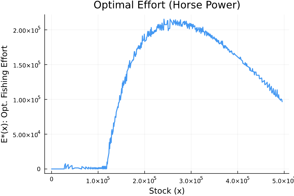
Figure 1: Optimal Effort as a Function of Fish Stock

The value function below confirms: more fish is generally better. But beyond a certain point (close to the carrying capacity $K$ ), the returns level off, since nature regulates the population growth.

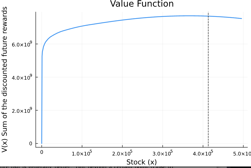
Figure 2: Value Function by Stock Level

6. Final Thoughts

This simple model captures the trade-off at the heart of sustainable resource use: harvest just enough today so that tomorrow's population—and profits—remain strong. While we used a basic setup here, this framework can easily be extended to include randomness, real data, or climate shocks.

Future posts will explore more complex models and estimation techniques. For now, you've seen how a classic economic tool can help us protect fish, profits, and the future.

This post demonstrates how dynamic programming transforms complex multi-period decisions into manageable recursive problems, providing a foundation for more sophisticated fisheries management models.

Code Implementation: I've provided the complete Julia code that implements this dynamic programming solution. The code includes value function iteration, optimal policy computation, and visualization of results.

Julia Implementation

#### Now optimal fisheries control in fisheries. ####
#### Author: Kyumin Kim ####
### Disclaimer: This is a simplified model for the purpose of showcasing optimal fisheries control.
### Feel free to use this code for your own research, but I do not guarantee the accuracy of the results.

# Load essential packages
using Random, Interpolations, Optim, LinearAlgebra, Statistics     # general-purpose numerical packages
using Interpolations: interpolate, Gridded, Linear                  # bring interpolation types into scope
using Plots                                                         # for graphing results

# -------------------------------
# 1. Model Parameters
# -------------------------------

r = 1.36            # Intrinsic growth rate of anchovy (biological parameter)
K = 4.13e5          # Carrying capacity (maximum population the environment can sustain)
q = 3.36e-6         # Catchability coefficient (how much fish are caught per unit effort)
p = 3050            # Fish price per ton
c = 280             # Cost per unit of fishing effort (e.g., fuel, labor)
β = 0.95            # Discount factor (how much future profits are valued)

# -------------------------------
# 2. Grid Setup
# -------------------------------

n = 600                                     # Number of grid points for fish stock (state space)
x_min = 10                                  # Minimum stock level (to avoid zero)
x_max = 1.2 * K                             # Maximum stock, allowing overshoot above carrying capacity
x_grid = range(x_min, x_max, length=n)      # Evenly spaced grid for stock levels

# Effort grid setup
m = 600                                     # Number of effort levels to consider (action space)
E_grid = range(0.0, stop=300000, length=m)  # Discrete levels of fishing effort (e.g., horsepower)

# -------------------------------
# 3. Initialize Value Function
# -------------------------------

V = zeros(n)            # Current value function V(x): value of being at stock x
E_opt = similar(V)      # Optimal policy: effort chosen at each x
V_new = similar(V)      # Placeholder to store updated value function in each iteration

# -------------------------------
# 4. Value Function Iteration Setup
# -------------------------------

max_iter = 1000         # Maximum number of iterations allowed
ϵ = 1e-4                # Convergence tolerance: stop when value function changes less than this

# Helper function: find the nearest grid point to a given value z
function findnearest(grid, z::Real)
    k = searchsortedfirst(grid, z)              # Find the insertion point in the sorted grid
    if k == 1
        return 1                                # If below the lowest point, return first index
    elseif k > length(grid)
        return length(grid)                     # If above the highest point, return last index
    else
        # Return whichever of grid[k] or grid[k-1] is closer to z
        return abs(grid[k] - z) < abs(grid[k - 1] - z) ? k : k - 1
    end
end

# -------------------------------
# 5. Value Function Iteration
# -------------------------------

for iter in 1:max_iter

    for i in 1:n
        x = x_grid[i]                # Current fish stock

        opt_value = -Inf            # Start with worst possible value
        opt_E = 0.0                 # Best effort found so far

        for j in 1:m
            E = E_grid[j]           # Try this effort level

            # Infeasibility check: you can't catch more fish than exist
            if q * x * E > x
                continue            # Skip this effort level if it violates feasibility
            end

            # Fish population transition: current + growth - harvest
            next_x = x + r * x * (1 - x / K) - q * x * E

            # Clamp to make sure next_x stays within grid bounds
            next_x = clamp(next_x, x_min, x_max)

            # Find the closest stock grid point to next_x
            next_nearest_value = findnearest(x_grid, next_x)
            V_next = V[next_nearest_value]   # Use value function at that nearest grid point

            # Immediate profit = revenue - cost
            current_reward = p * q * x * E - c * E

            # Bellman equation: total value = current reward + discounted future value
            value = current_reward + β * V_next

            # If this effort gives a higher value, update best value and best effort
            if value > opt_value
                opt_value = value
                opt_E = E
            end
        end

        # Store best value and policy at this stock level
        V_new[i] = opt_value
        E_opt[i] = opt_E
    end

    # Compute the max difference between old and new value function
    diff = maximum(abs.(V_new .- V))
    println("Difference: $diff")    # Show convergence progress

    # Stop if changes are small enough (converged)
    if diff < ϵ
        println("Converged in $iter iterations!, Kyumin is happy")
        break
    end

    V .= V_new    # Update value function for the next round
end

# -------------------------------
# 6. Plot Optimal Policy Function
# -------------------------------

# Plot: optimal fishing effort as a function of fish stock
p1 = plot(x_grid, E_opt,
          title = "Optimal Effort (Horse Power)",
          xlabel = "Stock (x)",
          ylabel = "E*(x): Opt. Fishing Effort",
          legend = false,
          lw = 2)
p1   # Display the plot

# -------------------------------
# 7. Plot Value Function
# -------------------------------

# Plot: total expected future reward at each stock level
p2 = plot(x_grid, V,
          title = "Value Function",
          xlabel = "Stock (x)",
          ylabel = "V(x): Sum of the discounted future rewards",
          legend = false,
          lw = 2)

# Add vertical dashed line at carrying capacity K
vline!(p2, [K],
       linestyle = :dash,
       color = :black,
       label = "Carrying Capacity")
p2   # Display the plot

# -------------------------------
# 8. Plot Logistic Growth Function (for illustration)
# -------------------------------

# Function to plot G(x) = r * x * (1 - x/K) and show MSY at K/2
function logistic_growth_plot(r::Real, K::Real; xmin = 0.0, xmax = 1.2K, n::Int = 400)
    x = collect(range(xmin, K; length = n))              # State grid
    G = r .* x .* (1 .- x ./ K)                          # Logistic growth values

    p = plot(x, G;
             lw      = 2,
             xlabel  = "Stock x",
             ylabel  = "Growth G(x)",
             title   = "Logistic Growth Function",
             legend  = false)

    # Add vertical dashed line at K/2 = MSY stock level
    vline!(p, [K / 2]; linestyle = :dash, color = :black, label = "")
    return p
end