Machine Learning Series 3: Decision Trees and Random Forests: A Friendly Introduction

Introduction

When people first learn machine learning, one of the most intuitive methods is the decision tree. A decision tree resembles a flowchart: you start at the top, answer a series of questions about your data, and end up with a prediction at the bottom. Despite their simplicity and interpretability, single decision trees often suffer from instability and limited predictive performance. This is where the random forest comes in — an ensemble method that combines many decision trees to create a more accurate and robust model.

Decision Trees: Classification and Regression Trees (CART)

A decision tree, often called a Classification and Regression Tree (CART), works by splitting the predictor space into smaller and smaller regions that best predict the outcome variable. For regression, the tree predicts the average value of the target $y$ in each region. For classification, the tree assigns the majority class.

How the Splitting Works

Suppose we have predictors $X = (X_1, X_2, \ldots, X_p)$, which may include continuous variables. At each step, the algorithm considers a variable $j$ and a split point $s$. This produces two regions:

For regression, the algorithm chooses $(j,s)$ to minimize the residual sum of squares (RSS):

where $\bar{y}_{R_k}$ is the mean of $y$ in region $R_k$.

This splitting is repeated recursively, so each region can be split again. The process stops when a criterion is reached (e.g., minimum node size). This approach is known as recursive binary splitting.

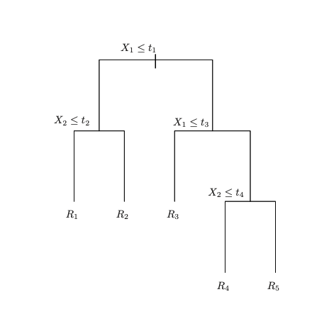
A regression tree representation.

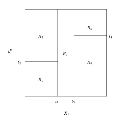
Partition of the predictor space.

Figure 1: Decision tree and corresponding partition of the predictor space. Left: a tree representation corresponding to the partition. Right: the output of recursive binary splitting on a two-dimensional example. Figure adapted from James et al. (2021).

Why "Greedy"?

The splitting process is called greedy because at each step, the algorithm chooses the split that gives the largest immediate reduction in prediction error, without considering whether a different split could lead to a better tree overall.

In other words, it optimizes locally, not globally. This makes the algorithm computationally feasible (since searching all possible trees is impossible), but also somewhat heuristic. Because of this greedy property, the choice of the first split can strongly influence the overall tree structure.

The Resulting Model

After $J$ splits, the predictor space is partitioned into $J$ disjoint rectangular regions $R_1, \ldots, R_J$. The prediction in each region is simply the mean (regression) or majority class (classification) of training observations in that region:

The fitted regression tree can then be written compactly as

where $1[X \in R_j]$ is an indicator function that equals 1 if $X$ falls in region $R_j$ and 0 otherwise. This representation shows that a regression tree is essentially a step function defined on regions of the predictor space.

Pros of Decision Trees

• Easy to interpret and visualize.
• Naturally handle both numerical and categorical data.
• Capture interactions between predictors automatically.

Cons of Decision Trees

• High variance: a small change in the data can lead to a very different tree.
• Greedy splitting may miss globally optimal structures.
• Often less accurate than more sophisticated models.

Random Forests

To address the weaknesses of single decision trees, the random forest was developed. A random forest is simply a collection of many decision trees, where each tree is built on a slightly different version of the data. The predictions are then averaged (for regression) or voted on (for classification).

How Random Forests Work

The name itself gives away the idea: a forest is simply a collection of trees. But why "random"? Because randomness is introduced in two ways:

1. Bootstrap sampling (bagging): Each tree is trained on a bootstrap sample of the data (random sample with replacement).
2. Random feature selection: At each split, only a random subset of predictors is considered, rather than all $p$ predictors. This decorrelates the trees, preventing them from all looking the same. A common rule of thumb is to use $m = \sqrt{p}$ predictors for classification problems, and $m \approx p/3$ for regression problems. The choice of $m$ can also be tuned as a hyperparameter.
3. Aggregation: For regression, predictions are averaged; for classification, predictions are based on majority vote.

Why They Work Better

• Averaging across many trees reduces variance, making predictions more stable and less sensitive to particular splits (such as the root choice).
• Random feature selection ensures diversity among trees, which further improves predictive accuracy.
• Random forests are robust to noise and perform well with high-dimensional predictor spaces.
• They provide measures of variable importance, helping to identify which predictors are most influential in determining the outcome.

When to Use Each Method

• Use a single decision tree when interpretability is most important, or as a quick baseline model.
• Use a random forest when prediction accuracy and robustness matter more than interpretability, especially with noisy or complex data.

Experimental Setup and Data Description

To demonstrate decision trees and random forests in practice, I use micro-level survey data from the 2003 U.S. Medical Expenditure Panel Survey (MEPS). The sample is restricted to individuals aged 65 to 90 years. This dataset is widely used in applied econometrics and health economics, as it provides rich information on demographics, health conditions, and medical expenditures.

The main outcome variable of interest is medical expenditure:

• totexp: total annual medical expenditure (continuous).

The set of predictors includes both continuous and binary variables.

Continuous predictors (xlist)

• income: annual household income (in thousands of dollars).
• educyr: years of education completed.
• age: age of the respondent (65--90).
• famsze: family size (number of household members).
• totchr: number of chronic medical conditions.

Binary predictors (dlist)

• suppins: has supplementary private insurance (=1 if yes).
• female: gender (=1 if female).
• white: race (=1 if White).
• hisp: ethnicity (=1 if Hispanic).
• marry: marital status (=1 if married).
• northe: region (=1 if Northeast).
• mwest: region (=1 if Midwest).
• south: region (=1 if South; West is the omitted baseline).
• msa: residence in a Metropolitan Statistical Area.
• phylim: has functional limitation.
• actlim: has activity limitation.
• injury: condition caused by accident or injury.
• priolist: has conditions on the medical priority list.
• hvgg: self-reported health is excellent, very good, or good.

This experimental setup allows me to illustrate how CART and Random Forests handle a mixture of continuous and categorical variables, while also highlighting the instability of single trees and the stability gained through averaging across many trees.

First, I created two single trees separately, each with a different random seed. I then analyzed which variables each tree identified as the most important determinants of seniors' medical expenditures.

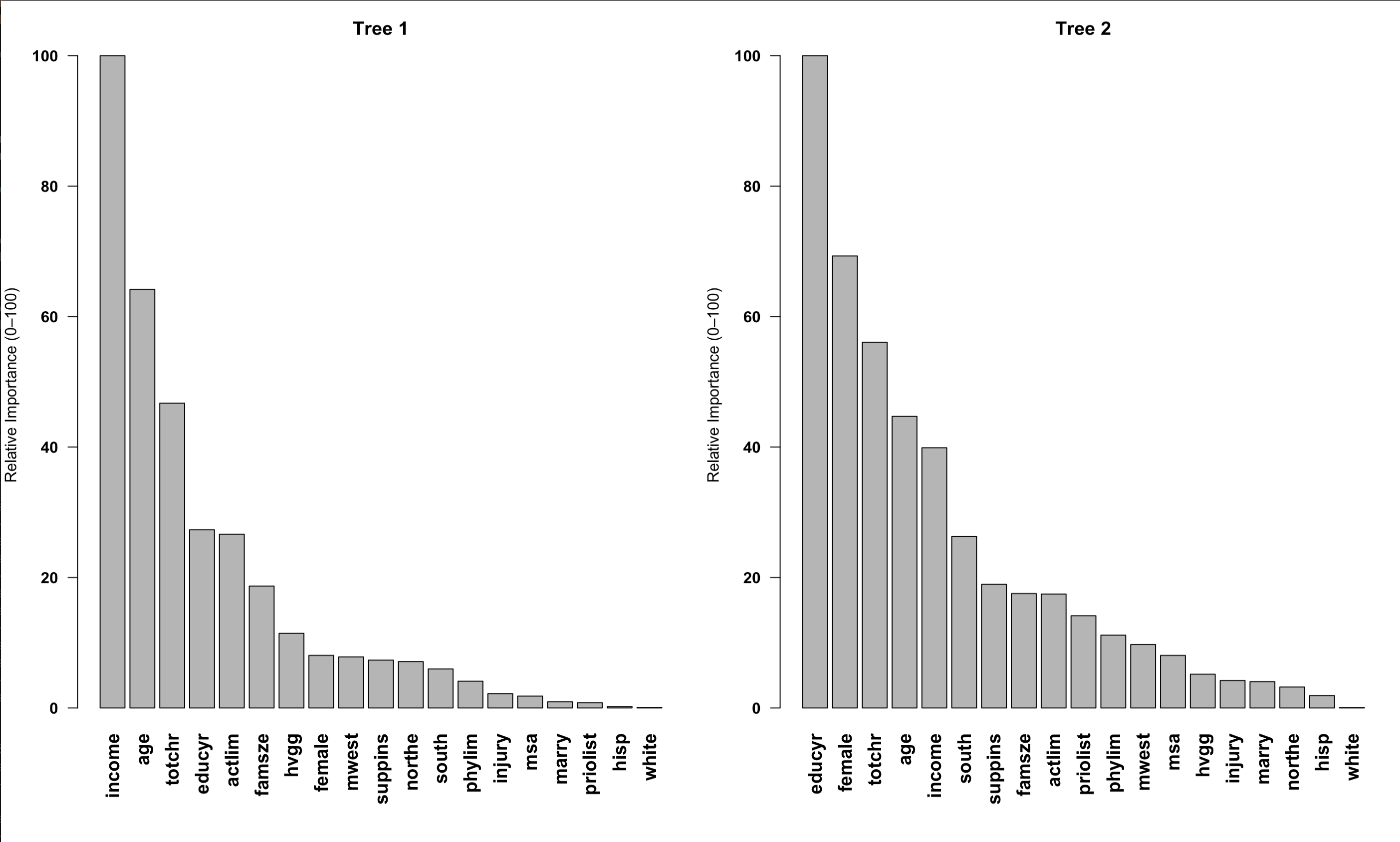
Figure 2: Single-tree based variable importance (rescaled between 1--100 for visibility).

As expected, single trees tell different stories. In the first tree, the top three important variables for medical expenditures are: income, age, and number of chronic conditions. In the second tree, however, education, gender, and number of chronic conditions are highlighted instead. The results vary considerably depending on the seed.

Next, I fit a random forest by growing up to 500 trees. The importance plot now clearly shows that income is the most relevant variable in predicting senior medical expenditures.

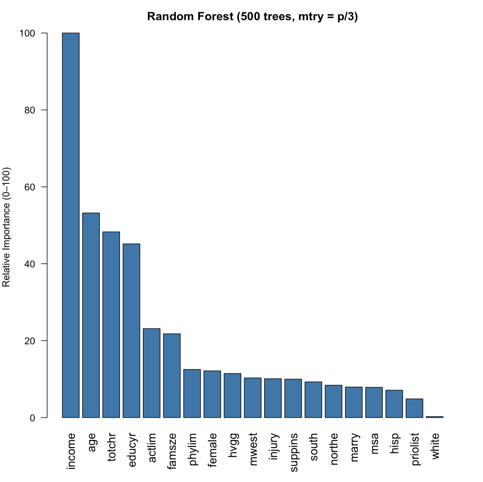
Figure 3: Random forest-based variable importance (rescaled between 1--100 for visibility).

Finally, what about prediction accuracy? At the beginning of the analysis, I split the data 50/50 into training and test samples. Using the test data for cross-validation, we can compare how well each model predicts actual outcomes. Figure 4 shows the prediction error computed by RMSE.

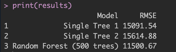
Figure 4: Prediction performance: RMSE comparison between single trees and random forest.

Not surprisingly, the random forest performs much better, as shown above. Why? Because each tree is a noisy estimator, but averaging multiple trees cancels out much of this noise. Think of it like one doctor's diagnosis versus 100 doctors' diagnoses averaged together. In addition, bagging and random predictor selection further improve performance. In short, while a single tree may have lower bias but high variance, the random forest slightly increases bias due to averaging, but drastically reduces variance.

Conclusion

Decision trees provide an intuitive and interpretable approach to machine learning, making them excellent for understanding data relationships and as baseline models. However, their high variance and instability often limit their predictive performance.

Random forests address these limitations by combining the strengths of multiple trees through ensemble methods. By introducing randomness in both data sampling and feature selection, random forests create diverse trees that, when averaged together, provide more stable and accurate predictions.

The experimental results with the MEPS dataset clearly demonstrate these principles: while individual trees show considerable variation in variable importance, the random forest provides consistent and reliable insights into the factors driving medical expenditures among seniors.

R Code Implementation

Below is the complete R code used to generate the analysis and figures presented in this post. This code demonstrates the practical implementation of decision trees and random forests using the MEPS dataset.

#####Kyumin Kim: Random Forest example #####

# Install if not already installed
#install.packages("haven") #For stata file load
# install.packages("randomForest")

rm(list=ls())

# install.packages(c("haven","dplyr","randomForest"))
library(haven)
library(dplyr)
library(randomForest)

# ---- Load & filter like Stata ("keep if ltotexp != ."). Original code made in STATA
dat <- read_dta("/Users/kyuminkim/Google Drive/ML example/mus203mepsmedexp.dta") %>%
  filter(!is.na(ltotexp))

# Quick look at structure
str(dat)
summary(dat)

# Predictors (X: cont. D: binary)
xlist <- c("income","educyr","age","famsze","totchr") ##Continous variable 
dlist <- c("suppins","female","white","hisp","marry","northe","mwest","south",
           "msa","phylim","actlim","injury","priolist","hvgg") #Binary dummy variable 
preds <- c(xlist, dlist) #All predictors 

# Drop IDs / constants
df <- dat %>%
  select(totexp, all_of(preds)) %>% #Choose outcome variables and 
  mutate(across(all_of(dlist), ~ as.factor(.)))  # binary to factors is ok for RF

# 50/50 split (Training and Validation)
set.seed(10101) #Random sampling for data split 

train_idx <- sample.int(nrow(df), size = floor(0.5 * nrow(df)))
train <- df[train_idx, ] # Tree traning 
test  <- df[-train_idx, ] #For cross-validation

#Number of predictors 
p <- length(preds)

# Helper: build ONE TREE with chosen seed, and get importance
fit_one_tree <- function(seed) {
  set.seed(seed)
  randomForest(
    totexp ~ ., data = train,
    ntree = 1,          # <-- single tree (like iter(1))
    mtry = p/3,         # <-- This is regression p/3
    nodesize = 5,       # <-- ~ lsize(5)
    maxnodes = 1024,    # <-- ~ depth(10) upper bound on leaves (2^10); not exact depth cap
    importance = TRUE,
    keep.forest = TRUE
  )
}

rf_seed_10101 <- fit_one_tree(10101)
rf_seed_1     <- fit_one_tree(1)

print(rf_seed_10101)
print(rf_seed_1)

# Variable importance (MeanDecreaseGini) & side-by-side barplots
imp1 <- importance(rf_seed_10101)[, "IncNodePurity"] ### Gini index mean decrease for regression 
imp2 <- importance(rf_seed_1)[, "IncNodePurity"]

# Order & simple threshold  (scale differs; keep top-k instead)
ord1 <- sort(imp1, decreasing = TRUE)
ord2 <- sort(imp2, decreasing = TRUE)

# Renormalize to 0–100 scale for easy relative importance 
scale_importance <- function(x) {
  100 * x / max(x, na.rm = TRUE)
}

ord1_scaled <- scale_importance(ord1)
ord2_scaled <- scale_importance(ord2)

op <- par(mfrow = c(1,2), mar = c(8,4,3,1))

barplot(ord1_scaled, las = 2, cex.names = 1.2, main = "Tree 1",
        ylab = "Relative Importance (0–100)",
        font.axis = 2)  # bold labels

barplot(ord2_scaled, las = 2, cex.names = 1.2, main = "Tree 2",
        ylab = "Relative Importance (0–100)",
        font.axis = 2)  # bold labels

par(op)

##Random forest with 500 trees

set.seed(10101)

mtry_p3 <- max(1, floor(p/3))  # regression rule-of-thumb

rf_200_p3 <- randomForest(
  totexp ~ ., data = train,
  ntree = 500,
  mtry = mtry_p3,
  nodesize = 5,
  importance = TRUE,
  keep.forest = TRUE
)

print(rf_200_p3)     # shows OOB MSE and % Var explained

### Variable importance 
# Variable importance (scaled 0–100)
imp_rf <- importance(rf_200_p3)
v <- sort(imp_rf[, "IncNodePurity"], decreasing = TRUE)

scale_importance <- function(x) 100 * x / max(x, na.rm = TRUE)
v_scaled <- scale_importance(v)

# Single barplot
barplot(v_scaled, las = 2, cex.names = 1.2,
        main = "Random Forest (500 trees, mtry = p/3)",
        ylab = "Relative Importance (0–100)", 
        col = "steelblue")

####Performance comparison for trees 1, 2 VS. random forest 

# ---- Helper RMSE function ----
rmse <- function(y, yhat) sqrt(mean((y - yhat)^2))

# ---- Predictions ----
pred_tree_10101 <- predict(rf_seed_10101, newdata = test)
pred_tree_1     <- predict(rf_seed_1,     newdata = test)
pred_rf_200     <- predict(rf_200_p3,     newdata = test)

# ---- Compute RMSE ----
rmse_tree_10101 <- rmse(test$totexp, pred_tree_10101)
rmse_tree_1     <- rmse(test$totexp, pred_tree_1)
rmse_rf_200     <- rmse(test$totexp, pred_rf_200)

# ---- Collect results ----
results <- data.frame(
  Model = c("Single Tree 1",
            "Single Tree 2",
            "Random Forest (500 trees)"),
  RMSE  = c(rmse_tree_10101, rmse_tree_1, rmse_rf_200)
)

print(results)