Today, I'm going to talk about shrinkage estimators, generally characterized as Ridge regression and the least absolute shrinkage and selection operator (LASSO), and Elastic Net (as a mix of Ridge and LASSO). What is shrinkage (or regularization)? That's what we're going to explore here.

Why do we use shrinkage methods?

Shrinkage—sometimes called regularization—is about reducing the influence of unnecessary variables in prediction.

High-dimensional (feature-rich) linear models often suffer from overfitting, where too many irrelevant variables are included. Overfitting increases the variance of estimates and hurts predictive accuracy.

Let's think about this in an economic or business prediction context:

Business example: Suppose a bank wants to determine whether a borrower will default on a loan. The bank has 50 different pieces of credit information about the borrower. Which variables actually contain meaningful predictive information?

Including all variables, even irrelevant ones, leads to overfitting and higher prediction variance. As we discussed in an earlier machine learning post, overfitting raises prediction error and reduces interpretability because you don't know which variables are truly important.

In general, machine learning methods allow some bias (unlike causal inference, which aims for unbiasedness) to achieve higher predictive accuracy by lowering variance. Shrinkage methods do exactly that: they deliberately pull coefficients of less relevant variables toward zero to stabilize estimates and improve out-of-sample prediction.

A toy example: when a biased estimator improves prediction

Let $\hat{\beta}_U$ be an unbiased estimator of $\beta$ :

E[\hat{\beta}_U] = \beta, \quad \mathrm{Var}(\hat{\beta}_U) = \sigma^2.

Then:

\mathrm{MSE}(\hat{\beta}_U) = \sigma^2.

Now consider a biased shrinkage estimator:

\hat{\beta}_S = k \, \hat{\beta}_U, \quad 0 \le k \le 1.

Bias:

\mathrm{Bias}(\hat{\beta}_S) = (k - 1)\beta.

Variance:

\mathrm{Var}(\hat{\beta}_S) = k^2 \sigma^2.

MSE:

\mathrm{MSE}(\hat{\beta}_S) = k^2 \sigma^2 + (k - 1)^2 \beta^2.

Shrinkage reduces MSE if:

\beta^2 < \frac{1 + k}{1 - k} \, \sigma^2.

Example:

If $k = 0.9$ , shrinkage improves MSE when:

\beta^2 < 19 \, \sigma^2.

Takeaway: Even though $\hat{\beta}_S$ is biased, the variance reduction can outweigh the squared bias, producing a smaller MSE and better prediction. This is the core logic behind Ridge regression and LASSO that I am going to introduce in the next part.

What do these shrinkage estimators look like?

Here I introduce three shrinkage estimators: Ridge, LASSO, and Elastic Net

These shrinkage methods minimize the residual sum of squares (like OLS) plus a penalty term.

Ridge regression (L2 penalty)

\hat{\beta}_\lambda = \argmin_{\beta}\;\frac{1}{n}\sum_{i=1}^n (y_i - x_i^\top \beta)^2 + \lambda\sum_{j=1}^p \beta_j^2.

The first term is the usual OLS loss. The second term, $\lambda\sum_{j=1}^p \beta_j^2$ , is the L2 penalty. A larger $\lambda$ penalizes large coefficients more strongly, shrinking them toward zero. Ridge never sets coefficients exactly to zero, making it useful when many predictors matter but when variables are highly correlated (like multicollinearity issue).

LASSO (L1 penalty)

\hat{\beta}_\lambda = \argmin_{\beta}\;\frac{1}{n}\sum_{i=1}^n (y_i - x_i^\top \beta)^2 + \lambda\sum_{j=1}^p |\beta_j|.

The L1 penalty can set coefficients exactly to zero, performing variable selection and improving interpretability.

Elastic Net (mix of L1 and L2)

\hat{\beta}_{\lambda,\alpha} = \argmin_{\beta}\;\frac{1}{n}\sum_{i=1}^n (y_i - x_i^\top \beta)^2 + \lambda\sum_{j=1}^p \left\{\alpha |\beta_j| + (1-\alpha)\beta_j^2\right\},

with $0\le \alpha \le 1$ . Setting $\alpha=1$ yields LASSO; $\alpha=0$ yields Ridge. Elastic Net is helpful when predictors are correlated, combining L2 stability with L1 sparsity.

How to choose a good $\lambda$ ?

In practice, you will naturally ask: How do we choose the shrinkage strength? The common approach is to use cross-validation to minimize the estimated out-of-sample loss. Algorithms in existing packages often search for the optimal $\lambda$ through a grid search. For each candidate $\lambda$ , they compute the mean squared error (MSE) and select the $\lambda$ that minimizes prediction error.

Alternatively, you can use information criteria, as in traditional econometrics. Common choices include the Bayesian Information Criterion (BIC), Akaike Information Criterion (AIC), and the Hannan–Quinn (HQ) criterion. BIC tends to favor more parsimonious models, while AIC, with its lighter penalty, generally allows more variables to remain in the model-fitting process. HQ is in the middle ground.

Adaptive LASSO and the oracle property

The adaptive LASSO extends LASSO to achieve the oracle property—the ability to select the true model with probability approaching one and to estimate coefficients as if the true model were known in advance. Basic LASSO does not have this property because its fixed penalty shrinks all nonzero coefficients equally, introducing bias.

Adaptive LASSO reweights the L1 penalty so that variables with stronger initial signals are penalized less. In plain language: you give more leniency to "well-behaved" variables (truly relevant predictors) while penalizing "misbehaving" variables (irrelevant predictors) more heavily.

Adaptive LASSO involves a two-step procedure:

Fit an initial model (often LASSO, but OLS is also possible) to obtain $\tilde{\beta}$ .
Define weights $w_j = 1/|\tilde{\beta}_j|^\delta$ for some $\delta>0$ and solve:

\hat{\beta}^{\text{AL}} = \argmin_{\beta}\;\frac{1}{n}\sum_{i=1}^n (y_i - x_i^\top \beta)^2 + \lambda\sum_{j=1}^p w_j |\beta_j|.

Under standard regularity conditions, adaptive LASSO achieves the oracle property.

R example: LASSO and adaptive LASSO with a known DGP

We simulate $X_1,\ldots,X_4$ , build $X_2X_3$ , and generate:

y = 3 + 1.5X_1 + 2X_2 + 3(X_2X_3) + \varepsilon,\quad \varepsilon\sim\mathcal{N}(0,\sigma^2).

We know the true predictors are $X_1$ , $X_2$ , and $X_2X_3$ . We compare LASSO and adaptive LASSO in small ( $n=30$ ) and large ( $n=500$ ) samples.

In LASSO, with the finite sample case $n=30$ , in reality, for instance, we actually do not know the true predictors. So, I run on all variables ( $X_1$ -- $X_4$ ) and their interaction terms:

y_i = \beta_0 + \sum_{j=1}^{4} \beta_j X_{ji} \;+\; \sum_{1 \le j < k \le 4} \beta_{jk} \, X_{ji} X_{ki} + \varepsilon_i

Then let's see how the LASSO estimation result looks under the finite sample case. I already found the optimal $\lambda$ by cross-validation at the lowest-MSE-achieving $\lambda$ , and under this $\lambda$ , we see the coefficient results for basic LASSO below.

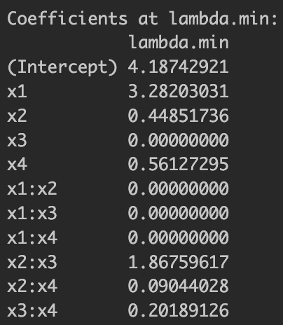
Basic LASSO estimation results showing coefficient values for different variables

Figure 1: Basic LASSO estimation results

We already know that the only relevant variables for $y$ are $X_1$ , $X_2$ , and $X_{2,3}$ . At least, it estimated larger coefficient values for the relevant variables but still included irrelevant variables. Now let's take a look at the result by adaptive LASSO below.

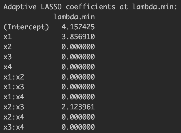
Adaptive LASSO estimation results showing more parsimonious variable selection

Figure 2: Adaptive LASSO estimation results

This time, it more parsimoniously selected variables but excluded $X_2$ . This more regularized model selection under adaptive LASSO is exactly what we expected.

Lastly, under a large sample size, I mentioned we would be able to see the "oracle property." I increased the sample size up to $n=700$ and re-ran adaptive LASSO. The results are shown below. Now you can see that the adaptive LASSO model under a large sample exactly chooses the true predictor variables. Adaptive LASSO's probability of selecting exactly the true predictors increases with $n$ , illustrating the oracle property. Plain LASSO may either omit relevant terms or include spurious ones.

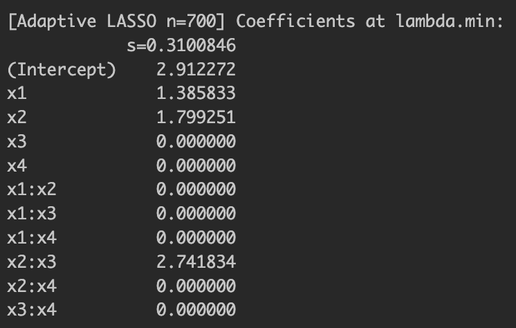
Adaptive LASSO estimation results demonstrating the oracle property with large sample size

Figure 3: Adaptive LASSO estimation results with oracle property

Takeaways

Shrinkage estimator trades bias for variance reduction to improve prediction.
Ridge is stable and keeps all variables. LASSO is sparse and performs selection. Elastic Net blends both.
Adaptive LASSO, through reweighted penalties, can recover the true model consistently and estimate it efficiently in large samples (of course, you should include all variables in the regression first).

R Implementation: Complete Code

Below is the complete R code used to generate the results shown in the figures above. This implementation demonstrates LASSO, adaptive LASSO, and shows the oracle property with different sample sizes.

### Kyumin Kim: Ridge, LASSO, and adaptive LASSO

rm(list=ls())

###############################################
# LASSO with pairwise interactions (x1..x4)
# Finite-sample evaluation with n_fit = 40
###############################################

library(glmnet)

set.seed(2025)

# ---------- 1) DGP: correlated predictors ----------
n  <- 1000        # total sample size
p  <- 4          # number of base predictors (x1..x4)
rho <- 0.4       # target pairwise correlation (population level)

# Simple common-factor generator for correlation
a <- sqrt(rho)                   # loading on common factor
b <- sqrt(1 - rho)               # loading on idiosyncratic noise
s <- rnorm(n)                    # common factor (length n)
E <- matrix(rnorm(n * p), n, p)  # idiosyncratic noise

X0 <- a * s + b * E              # each column has Corr ≈ rho with others
colnames(X0) <- paste0("x", 1:p)

# Extract predictors
x1 <- X0[, 1]; x2 <- X0[, 2]; x3 <- X0[, 3]; x4 <- X0[, 4]

# True DGP for y uses intercept, x1, x2, and x2:x3
x2x3 <- x2 * x3
beta_true <- c("(Intercept)"=3, "x1"=1.5, "x2"=2, "x3"=0, "x4"=0, "x2:x3"=3)
sigma_eps <- 4

y <- beta_true["(Intercept)"] +
  beta_true["x1"] * x1 +
  beta_true["x2"] * x2 +
  beta_true["x2:x3"] * x2x3 +
  rnorm(n, 0, sigma_eps)

# ---------- 2) Design matrix with ONLY pairwise interactions ----------
# (x1 + x2 + x3 + x4)^2 expands to mains + all 2-way interactions.
# "- 1" removes the intercept since glmnet handles it internally.
dat <- data.frame(x1 = x1, x2 = x2, x3 = x3, x4 = x4)
form_pair <- ~ (x1 + x2 + x3 + x4)^2 - 1
X_pair <- model.matrix(form_pair, data = dat)

# Sanity check: 4 mains + 6 pairwise = 10 columns
cat("Number of features (pairwise):", ncol(X_pair), "\n")
# cat("Feature names:\n"); print(colnames(X_pair))  # uncomment if you want to see them

# ---------- 3) Subsample to n_fit = 40: I want to see finite sample case first ----------
set.seed(2025)
n_fit <- 30
idx   <- sample.int(nrow(X_pair), n_fit, replace = FALSE)

X_fit <- X_pair[idx, , drop = FALSE]
y_fit <- y[idx]

# ---------- 4) LASSO with cross-validation to find the best regulation strength ----------
set.seed(2025)
cv_lasso <- cv.glmnet(
  x = X_fit,
  y = y_fit,
  alpha  = 1,          # LASSO
  family = "gaussian",
  nfolds = 5           # 5-fold CV for n_fit = 40
  # standardize = TRUE by default
)

# Optimal lambdas
lambda_min <- cv_lasso$lambda.min   # minimizes mean CV error
cat("\nLASSO CV:\n  lambda.min =", lambda_min)

# Coefficients at each chosen lambda through K-fold CV

coef_min <- as.matrix(coef(cv_lasso, s = "lambda.min"))
cat("\nCoefficients at lambda.min:\n"); print(coef_min)

# Selected variables (non-zero, excluding the intercept)
sel_min <- setdiff(rownames(coef_min)[as.numeric(coef_min) != 0], "(Intercept)")
cat("\nSelected at lambda.min:",
    if (length(sel_min)) paste(sel_min, collapse = ", ") else "(none)", "\n")


# ---------- 5) Adaptive LASSO (no Ridge; LASSO-initial) ----------
# Step 1: initial LASSO to get starting coefficients
set.seed(2025)
cv_init_lasso <- cv.glmnet(
  x = X_fit,
  y = y_fit,
  alpha  = 1,          # LASSO
  family = "gaussian",
  nfolds = 5
)

# Extract initial coefs at lambda.min (includes intercept in the first entry)
beta_init <- as.numeric(coef(cv_init_lasso, s = "lambda.min"))
names(beta_init) <- rownames(coef(cv_init_lasso, s = "lambda.min"))

# Step 2: build adaptive weights for features (exclude intercept)
# Handle zeros by adding a small epsilon; optionally cap very large weights.
delta_adapt <- 1.0
beta0 <- beta_init[-1]  # drop intercept
eps_small <- max(1e-6, 1e-6 * max(abs(beta0)))  # scale-aware epsilon. Let's avoide NaN
w_adapt <- 1 / (abs(beta0)^delta_adapt + eps_small)


# Step 3: fit weighted (adaptive) LASSO
set.seed(2025)
cv_adalasso <- cv.glmnet(
  x = X_fit,
  y = y_fit,
  alpha          = 1,              # LASSO objective
  family         = "gaussian",
  nfolds         = 5,
  penalty.factor = w_adapt         # feature-specific penalties
  # Intercept is not penalized by default
)


# Results at the chosen lambda
lambda_min_adapt <- cv_adalasso$lambda.min
cat("\nAdaptive LASSO: lambda.min =", lambda_min_adapt, "\n")

adalasso_min <- as.matrix(coef(cv_adalasso, s = "lambda.min"))
cat("\nAdaptive LASSO coefficients at lambda.min:\n"); print(adalasso_min)

# Selected variables (non-zero, excluding the intercept)
sel_adapt <- setdiff(rownames(adalasso_min)[as.numeric(adalasso_min) != 0], "(Intercept)")
cat("\nAdaptive LASSO selected (lambda.min):",
    if (length(sel_adapt)) paste(sel_adapt, collapse = ", ") else "(none)", "\n")

# ---------- 6) Plots (optional) ----------
par(mfrow = c(1, 2))
plot(cv_init_lasso, main = "Initial LASSO CV")
plot(cv_adalasso,  main = "Adaptive LASSO CV")
par(mfrow = c(1, 1))




######## Now do the same for adaptive LASSO but when n=450 not 30 any longer.
#
#
#. ########### To show Oracle property of Adpative LASSO. 
#
#
###########################################################

######## Use n_fit = 700 (full-sample permutation)

# 1) Subsample to n_fit = 700, Well I initially started with n=500, changed value.
set.seed(2026)  # different seed so this draw is independent of the n=30 case
n_fit_500 <- 700
idx_500   <- sample.int(nrow(X_pair), n_fit_500, replace = FALSE)

X_fit_500 <- X_pair[idx_500, , drop = FALSE]
y_fit_500 <- y[idx_500]

# 2) LASSO with cross-validation (only lambda.min)
set.seed(2026)
cv_lasso_500 <- cv.glmnet(
  x = X_fit_500,
  y = y_fit_500,
  alpha  = 1,           # LASSO
  family = "gaussian",
  nfolds = 5
)

lambda_min_500 <- cv_lasso_500$lambda.min
cat("\n[LASSO n=700] lambda.min =", lambda_min_500, "\n")

# 3) Adaptive LASSO (LASSO-initial, no Ridge)
# Use the LASSO fit above for initial coefficients
beta_init_500 <- as.numeric(coef(cv_lasso_500, s = lambda_min_500))  # includes intercept
names(beta_init_500) <- rownames(coef(cv_lasso_500, s = lambda_min_500))

# Build adaptive weights (exclude intercept)
delta_adapt <- 1.0
beta0_500   <- beta_init_500[-1]
eps_small_500 <- max(1e-6, 1e-6 * max(abs(beta0_500)))  # avoid infinite weights
w_adapt_500 <- 1 / (abs(beta0_500)^delta_adapt + eps_small_500)

# Fit adaptive LASSO
set.seed(2026)
cv_adalasso_500 <- cv.glmnet(
  x = X_fit_500,
  y = y_fit_500,
  alpha          = 1,
  family         = "gaussian",
  nfolds         = 5,
  penalty.factor = w_adapt_500     # weighted penalty for adaptive LASSO
)

lambda_min_adapt_500 <- cv_adalasso_500$lambda.min
cat("\n[Adaptive LASSO n=700] lambda.min =", lambda_min_adapt_500, "\n")

coef_adalasso_min_500 <- as.matrix(coef(cv_adalasso_500, s = lambda_min_adapt_500))
cat("\n[Adaptive LASSO n=700] Coefficients at lambda.min:\n"); print(coef_adalasso_min_500)

sel_adapt_500 <- setdiff(rownames(coef_adalasso_min_500)[as.numeric(coef_adalasso_min_500) != 0], "(Intercept)")
cat("\n[Adaptive LASSO n=700] Selected at lambda.min:",
    if (length(sel_adapt_500)) paste(sel_adapt_500, collapse = ", ") else "(none)", "\n")

#Apology for my laziness for not changing objects' names. 
# 
# # 4) Optional plots for the n=100 case
# par(mfrow = c(1, 2))
# plot(cv_lasso_100,    main = "LASSO CV (n_fit = 100)")
# plot(cv_adalasso_100, main = "Adaptive LASSO CV (n_fit = 100)")
# par(mfrow = c(1, 1))
#

Note: This R code demonstrates the complete implementation of LASSO and adaptive LASSO with cross-validation, showing both finite sample behavior (n=30) and the oracle property with larger samples (n=700). The code includes data generation, model fitting, and result visualization.

A Friendly Introduction to Shrinkage Estimators: Ridge, LASSO, Elastic Net, and the Adaptive LASSO